Stephen Rolt - Optical Engineering Science
Здесь есть возможность читать онлайн «Stephen Rolt - Optical Engineering Science» — ознакомительный отрывок электронной книги совершенно бесплатно, а после прочтения отрывка купить полную версию. В некоторых случаях можно слушать аудио, скачать через торрент в формате fb2 и присутствует краткое содержание. Жанр: unrecognised, на английском языке. Описание произведения, (предисловие) а так же отзывы посетителей доступны на портале библиотеки ЛибКат.
- Название:Optical Engineering Science
- Автор:
- Жанр:
- Год:неизвестен
- ISBN:нет данных
- Рейтинг книги:3 / 5. Голосов: 1
-
Избранное:Добавить в избранное
- Отзывы:
-
Ваша оценка:
Optical Engineering Science: краткое содержание, описание и аннотация
Предлагаем к чтению аннотацию, описание, краткое содержание или предисловие (зависит от того, что написал сам автор книги «Optical Engineering Science»). Если вы не нашли необходимую информацию о книге — напишите в комментариях, мы постараемся отыскать её.
Offers a comprehensive review of the topic of optical engineering Covers topics such as optical fibers, waveguides, aspheric surfaces, Zernike polynomials, polarisation, birefringence and more Targets engineering professionals and students Filled with illustrative examples and mathematical equations Written for professional practitioners, optical engineers, optical designers, optical systems engineers and students,
offers an authoritative guide that covers the broad range of optical design and optical metrology topics and their applications.
Optical Engineering Science — читать онлайн ознакомительный отрывок
Ниже представлен текст книги, разбитый по страницам. Система сохранения места последней прочитанной страницы, позволяет с удобством читать онлайн бесплатно книгу «Optical Engineering Science», без необходимости каждый раз заново искать на чём Вы остановились. Поставьте закладку, и сможете в любой момент перейти на страницу, на которой закончили чтение.
Интервал:
Закладка:
The two square root terms represent the optical path of two ‘legs’ of the journey, with the path through the glass adding a multiplicative factor of n. The next stage of the process is an extension of the paraxial theory. It is assumed that r x, r y, and u θ are all significantly less than u . We can now approximate Φ from Eq. (4.2)using the binomial theorem. In the meantime collecting terms we get:

Before deriving the third order aberration terms, we examine the paraxial contribution which contain terms in h up to order r 2.
(4.3) 
As one would expect, in the paraxial approximation, the optical path length is identical for all rays. However, for third order aberration, terms of up to order h 4must be considered. Expanding Eq. (4.2)to consider all relevant terms, we get:
(4.4) 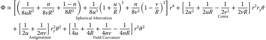
Four of the five Gauss-Seidel terms are present – spherical aberration, coma, astigmatism, and field curvature. However, clearly there is no distortion. In fact, as will be seen later, distortion can only occur where the stop is not at the surface as it is here. Of course, Eq. (4.4)can be simplified if one considers that u, v, and R are dependent variables, as related in Eq. (4.3). Substituting v for u , and R , we can express the OPD in terms of u and R alone. Furthermore, it is useful, at this stage to split the OPD contributions in Eq. (4.4)into Spherical Aberration (SA), Coma (CO), Astigmatism (AS), and Field Curvature (FC). With a little algebraic manipulation this gives:
(4.5a) 
(4.5b) 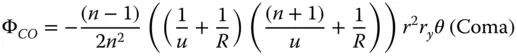
(4.5c) 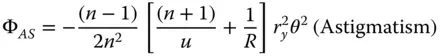
(4.5d) 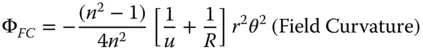
4.2.1 Aplanatic Points
It is worthwhile, at this juncture, to examine the four expressions in Eqs. (4.5a)– (4.5d)in some detail and, in particular, those for spherical aberration and coma. Before examining these expressions further, it is worthwhile to cast them in the form outlined in Chapter 3:
(4.6a) 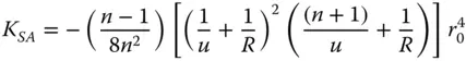
(4.6b) 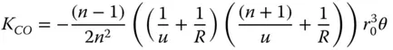
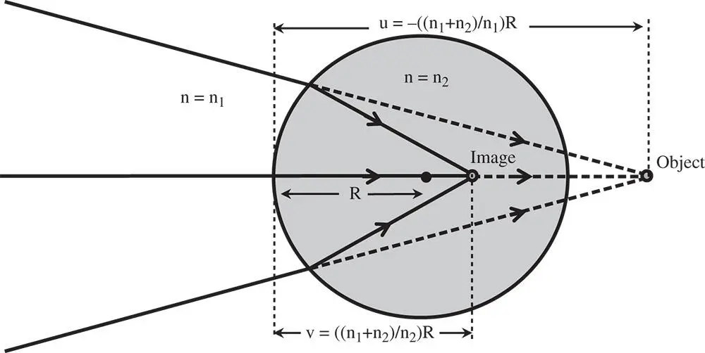
Figure 4.2 Aplanatic points for refraction at single spherical surface.
There is a clear pattern in these expressions in that both spherical aberration and coma can be reduced to zero for specific values of the object distance, u . Examining Eqs. (4.6a)and (4.6b), it is evident that this condition is met where u = − R . That is to say, where the object is located at the centre of the spherical surface. However, this is a somewhat trivial condition where rays are undeviated by the surface and where the surface would not provide any useful additional refractive power to the system. Most significantly, another condition does exist for u = −( n + 1) R . Here, for this non-trivial case, both third order spherical aberration and coma are absent. This is the so-called aplanatic conditionand the corresponding conjugate points are referred to as aplanatic points( Figure 4.2). From Eq. (4.3)we can derive the image distance, v , as ( n + 1) R / n . That is to say, the object is virtual and the image is real if R is positive and vice-versa if R is negative.
To be a little more rigorous, we might suppose that refractive index in object space is n 1and that in image space is n 2. The location of the aplanatic points is then given by:
(4.7) 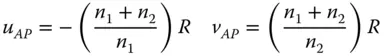
Fulfilment of the aplanatic condition is an important building block in the design of many optical systems and so is of great practical significance. As pointed out in the introduction, for those systems where the field angles are substantially less than the marginal ray angles, such as microscopes and telescopes, the elimination of spherical aberration and coma is of primary importance. Most significantly, not only does the aplanatic condition eliminate third order spherical aberration, but it also provides theoretically perfect imaging for on axis rays.
Worked Example 4.1 Microscope Objective
The ‘front end’ of many high power microscope objectives exploits the principle of single surface aplanatic points through the use of a hyperhemisphere co-located with the object. The hyperhemisphere consists of a sphere that has been truncated at one of the aplanatic points which also coincides with the object location, as illustrated in Figure 4.3.
Using the hyperhemisphere, we wish to create a ×20 microscope objective for a standard optical tube length of 200 mm. In this example, it is assumed that two thirds of the optical power resides in the hyperhemisphere itself; other components collimate the beam. In other words:
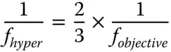
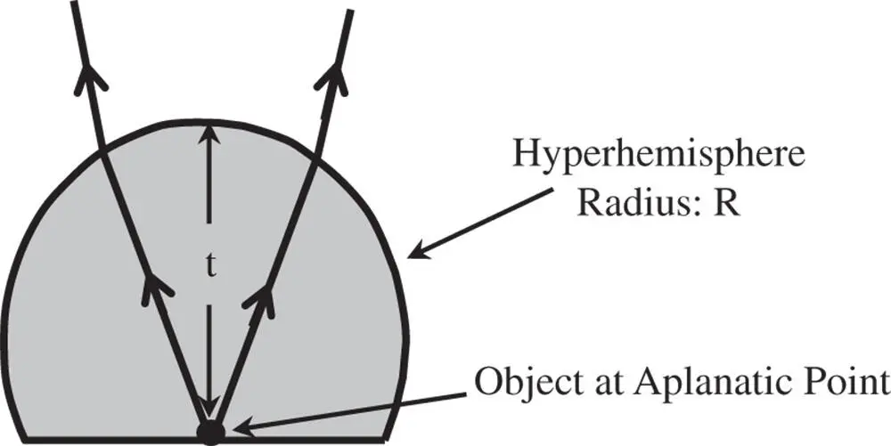
Figure 4.3 Hyperhemisphere objective.
The refractive index of the hyperhemisphere is 1.6. What is the radius, R , of the hyperhemisphere and what is its thickness?
For a tube length of 200 mm, a ×20 magnification corresponds to an objective focal length of 10 mm. As two thirds of the power resides in the hyperhemisphere, then the focal length of the hyperhemisphere must be 15 mm. Inspecting Figure 4.2, it is clear that the thickness of the hyperhemisphere is − R × ( n + 1)/ n , or −1.625 × R . To calculate the value of R , we set up a matrix for the system. The first matrix corresponds to refraction at the planar air/glass boundary, the second to translation to the spherical surface and the final matrix to the refraction at that surface. On this occasion, translation to the original reference is not included.
Читать дальшеИнтервал:
Закладка:
Похожие книги на «Optical Engineering Science»
Представляем Вашему вниманию похожие книги на «Optical Engineering Science» списком для выбора. Мы отобрали схожую по названию и смыслу литературу в надежде предоставить читателям больше вариантов отыскать новые, интересные, ещё непрочитанные произведения.


Обсуждение, отзывы о книге «Optical Engineering Science» и просто собственные мнения читателей. Оставьте ваши комментарии, напишите, что Вы думаете о произведении, его смысле или главных героях. Укажите что конкретно понравилось, а что нет, и почему Вы так считаете.