Zhuming Bi - Computer Aided Design and Manufacturing

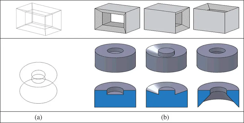
Figure 2.23Ambiguity examples of wireframe models. (a) Wireframe model. (b) Possible solid geometries.

On the other hand, a wireframe model is very concise and fundamental. It can be used as the supporting technique for other modelling methods.

Surface modelling aims to create the models for finite, non‐open surface patches of free forms. Note that the boundary surfaces of an object are formed by positioning and joining surface patches with the specified continuity restrictions. A surface modelling method does not represent the topological information of geometric elements such as knitting of boundary surfaces into a watertight volume. Figure 2.24shows an example of a modelled surface from the surface modelling method. A surface model differs from a solid model since there is no information of the thickness.

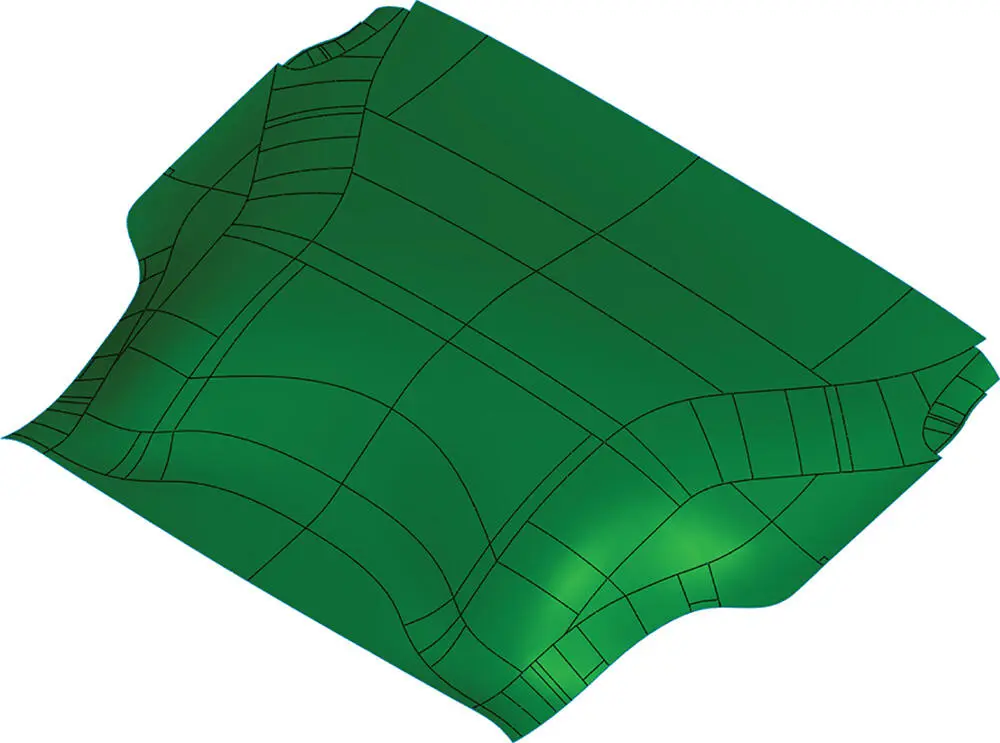
Figure 2.24Surface model example.

Differing from a wireframe model, a surface model has sufficient information to determine hide and shade displays when multiple surfaces are involved; however, a surface model does not include information of volumes or masses. Therefore, it is usually unsuitable to be used in simulations for engineering analysis unless the object is a sheet part with uniform thickness perpendicular to surfaces.

Boundary surface modelling (B‐Rep) is used to define the finite and closed cover of an object (the mantle) upon a surface model. In B‐Rep modelling, it is assumed that each physical object has an unambiguously determinable boundary surface, which is a continuous closing set of surface patches. Since a finite volume is defined, the B‐Rep method provides a comprehensive topological characterization of solids.

In defining the volume of solids, B‐Rep modelling utilizes a surface model with all of its determined boundary surface patches, and the normal vector of each surface patch is then determined. A watertight volume can be finally determined by collecting all spatial points at the internal sides of all the surrounding boundary surfaces. This is implemented by the half‐space concept.

Mathematically, a half space can be expressed as

(2.17)

which shows that point P belongs to a half space E 3if the condition f ( P ) < 0 can be satisfied where f ( P ) = 0 is the equation of the surface in an implicit form. The examples of surface equations for some common geometric elements are given in Table 2.10.

Table 2.10Equations of common surfaces.

Name	Illustration	Implicit equation f ( P ) = 0
Flat XY plane		{( x , y , z ) : z = d }
Cylinder		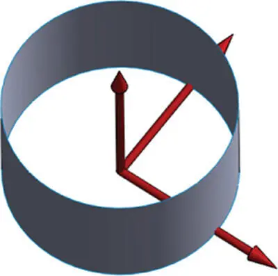{( x , y , z ) : x 2+ y 2= R 2}
Cone		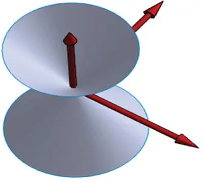{( x , y , z ) : x 2+ y 2= kz 2}
Sphere		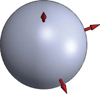{( x , y , z ) : x 2+ y 2+ z 2= R 2}
Torus		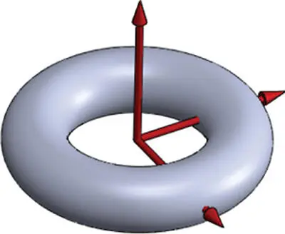{( x , y , z ) : ( x 2+ y 2+ z 2− R 2 2− R 2 1) 2= 4 R 2 2( R 2 1− z 2)}

The half space on one side of the surface is empty while the other one is filled with a material. The B‐Rep method assumes that the volume occupied by an object is bounded by surfaces of infinite extension. Each surface divides space into two regions of infinite extension. The volume of the solid S is the intersection (common portion) of half spaces H i( i = 1, 2 , …, N ) where

(2.18)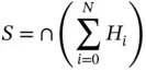

Figure 2.25shows an example where the B‐Rep method is applied to define a rectangle body ( Figure 2.25b) as an intersected volume of seven surfaces of infinite extension ( left , right , rear , front , top , bottom , and central cylinder ) ( Figure 2.25a).

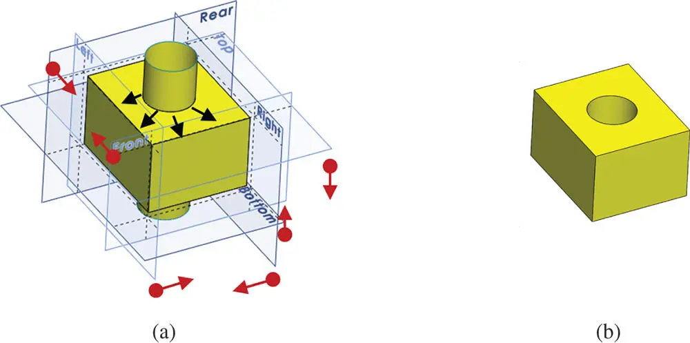
Figure 2.25Example of half‐spaces in B‐Rep method. (a) Seven surfaces with an infinite extension. (b) Enclosed volume by seven half spaces.

In a space decomposition, an object is represented by a collection of isomorphic cells. The sizes of isomorphic cells are very small, being several orders of the magnitude smaller than the dimensions of an object. The space decomposition method is very popular in numerical simulations such as finite element analysis and boundary element analysis .

Figure 2.26illustrate how the space decomposition is processed as well as the corresponding data structure. The space decomposition is performed as the following procedure:

1 It divides a finite space into eight parts (producing octants).

2 It then examines each space region as to whether they are fully or partly filled.

3 Partial regions that are totally filled up or are not filled at all can be excluded from further investigations.

4 The partially filled octants are continuously refined until the required accuracy is achieved.

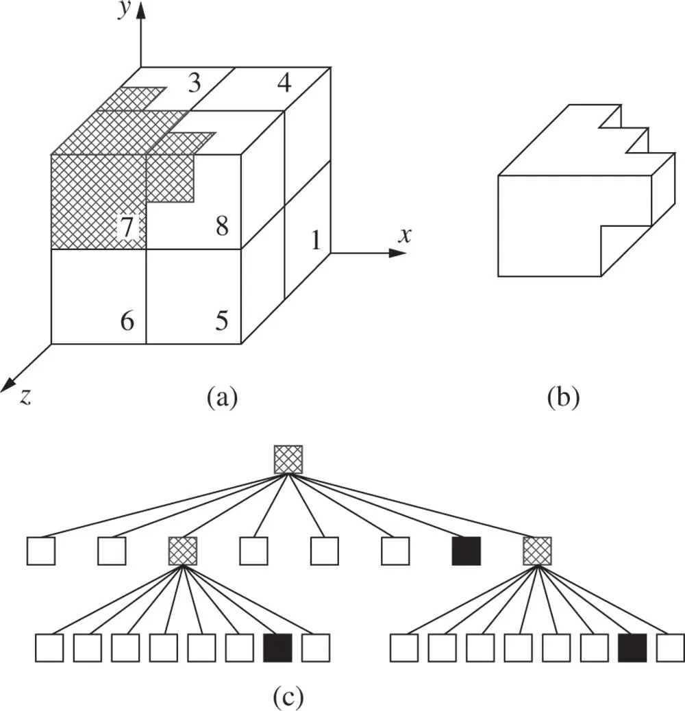
Figure 2.26Data structure of space composition.

Figure 2.27shows examples of using the space decomposition method to represent objects (Bi and Kang 2014). In the left column, the datasets of point clouds are obtained by 3D scanning, and in the right column, the point clouds have been transformed into solid geometries using the space decomposition method.

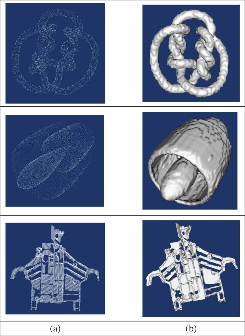
Figure 2.27Examples of solid objects using a space decomposition method (Bi and Kang 2014). (a) Point cloud datasets of objects. (b) Solids and surfaces from the space decomposition method.