Won Y. Yang - Applied Numerical Methods Using MATLAB
Здесь есть возможность читать онлайн «Won Y. Yang - Applied Numerical Methods Using MATLAB» — ознакомительный отрывок электронной книги совершенно бесплатно, а после прочтения отрывка купить полную версию. В некоторых случаях можно слушать аудио, скачать через торрент в формате fb2 и присутствует краткое содержание. Жанр: unrecognised, на английском языке. Описание произведения, (предисловие) а так же отзывы посетителей доступны на портале библиотеки ЛибКат.
- Название:Applied Numerical Methods Using MATLAB
- Автор:
- Жанр:
- Год:неизвестен
- ISBN:нет данных
- Рейтинг книги:5 / 5. Голосов: 1
-
Избранное:Добавить в избранное
- Отзывы:
-
Ваша оценка:
Applied Numerical Methods Using MATLAB: краткое содержание, описание и аннотация
Предлагаем к чтению аннотацию, описание, краткое содержание или предисловие (зависит от того, что написал сам автор книги «Applied Numerical Methods Using MATLAB»). Если вы не нашли необходимую информацию о книге — напишите в комментариях, мы постараемся отыскать её.
Applied Numerical Methods Using MATLAB®, Second Edition Provides examples and problems of solving electronic circuits and neural networks Includes new sections on adaptive filters, recursive least-squares estimation, Bairstow's method for a polynomial equation, and more Explains Mixed Integer Linear Programing (MILP) and DOA (Direction of Arrival) estimation with eigenvectors Aimed at students who do not like and/or do not have time to derive and prove mathematical results
is an excellent text for students who wish to develop their problem-solving capability without being involved in details about the MATLAB codes. It will also be useful to those who want to delve deeper into understanding underlying algorithms and equations.
Applied Numerical Methods Using MATLAB — читать онлайн ознакомительный отрывок
Ниже представлен текст книги, разбитый по страницам. Система сохранения места последней прочитанной страницы, позволяет с удобством читать онлайн бесплатно книгу «Applied Numerical Methods Using MATLAB», без необходимости каждый раз заново искать на чём Вы остановились. Поставьте закладку, и сможете в любой момент перейти на страницу, на которой закончили чтение.
Интервал:
Закладка:
Note that we can define a simple function not only in an independent M‐file but also inside a script by using the function handle operator @, the ‘ inline()’ command, or just in a form of literal expression that can be evaluated by the command ‘ eval()’.
>f1h=@(x)1./(1+8*x.̂2); % Using function handle >f1i=inline('1./(1+8*x.̂2)','x'); % Usng inline() >f1h([0 1]), feval(f1h,[0 1]), f1i([0 1]), feval(f1i,[0 1]) ans= 1.0000 0.1111 ans= 1.0000 0.1111 >f1='1./(1+8*x.̂2)'; x=[0 1]; eval(f1) ans= 1.0000 0.1111
As far as a polynomial function is concerned, it can simply be defined as its coefficient vector arranged in descending order. It may be called to yield its value for certain value(s) of its independent variable by using the command ‘ polyval()’.
>p=[1 0 –3 2]; % Polynomial function p(x) = x3-3x + 2 >polyval(p,[0 1]) % Polynomial function values at x=0 and 1 ans= 2.0000 0.0000
The multiplication of two polynomials can be performed by taking the convolution of their coefficient vectors representing the polynomials in MATLAB, since

where

This operation can be done by using the MATLAB built‐in command ‘ conv()’ as illustrated beneath:
>a=[1 –1]; b=[1 1 1]; c=conv(a,b) c= 1 0 0 -1 % meaning that (x-1)(x2 + x + 1) = x3 + 0 ⋅ x2 + 0 ⋅ x-1
But, in case you want to multiply a polynomial by only x n, you can simply append n zeros to the right end of the polynomial coefficient vector to extend its dimension.
>a=[1 2 3]; c=[a 0 0] % equivalently, c=conv(a,[1 0 0]) c= 1 2 3 0 0 % meaning that (x2 + 2x + 3)x2 = x4 + 2x3 + 3x2 + 0 ⋅ x + 0
1.1.7 Operations on Vectors and Matrices
We can define a new scalar/vector/matrix or redefine any existing ones in terms of the existent ones or irrespective of them. In the MATLAB Command window, let us define A and B as
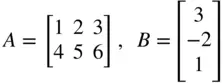
by running
>A=[1 2 3;4 5 6], B=[3;-2;1]
We can modify them or take a portion of them. For example:
>A=[A;7 8 9] A= 1 2 3 4 5 6 7 8 9 >B=[B [1 0 -1]'] B= 3 1 -2 0 1 -1
Here, the apostrophe (prime) operator ( ') takes the complex conjugate transpose and functions virtually as a transpose operator for real‐valued matrices. If you want to take just the transpose of a complex‐valued matrix, you should put a dot ( .) before ', i.e. ‘ .'’.
When extending an existing matrix or defining another one based on it, the compatibility of dimensions should be observed. For instance, if you try to annex a 4 × 1 matrix into the 3 × 1 matrix B, MATLAB will reject it squarely, giving you an error message.
>B=[B ones(4,1)] Error using horzcat Dimensions of matrices being concatenated are not consistent.
We can modify or refer to a portion of a given matrix.
>A(3,3)=0 A= 1 2 3 4 5 6 7 8 0 >A(2:3,1:2) % from 2nd row to 3rd row, from 1st column to 2nd column ans= 4 5 7 8 >A(2,:) % 2nd row, all columns ans= 4 5 6
The colon ( :) is used for defining an arithmetic (equal difference) sequence without the bracket []as
>t=0:0.1:2
which makes
t=[0.0 0.1 0.2 … 1.9 2.0]
1 (Q8) What if we omit the increment between the left/right boundary numbers?
2 (A8) By default, the increment is 1.>t=0:2 t= 0 1 2
3 (Q9) What if the right boundary number is smaller/greater than the left boundary number with a positive/negative increment?
4 (A9) It yields an empty matrix, which is useless.>t=0:-2 t= Empty matrix: 1-by-0
5 (Q10) If we define just some elements of a vector not fully, but sporadically, will we have a row vector or a column vector and how will it be filled in between?
6 (A10) We will have a row vector filled with zeros between the defined elements.>D(2)=2; D(4)=3 D= 0 2 0 3
7 (Q11) How do we make a column vector in the same style?
8 (A11) We must initialize it as a (zero‐filled) row vector, prior to giving it a value.>D=zeros(4,1); D(2)=2; D(4)=3 D= 0 2 0 3
9 (Q12) What happens if the specified element index of an array exceeds the defined range?
10 (A12) It is rejected. MATLAB does not accept nonpositive or noninteger indices.>D(5) Index exceeds matrix dimensions. >D(0)=1; Subscript indices must either be real positive integers or logicals. >D(1.2) Subscript indices must either be real positive integers or logicals.
11 (Q13) How do we know the size (the numbers of rows/columns) of an already‐defined array?
12 (A13) Use the ‘ length()’, ‘ size()’, and ‘ numel()’ commands as indicated as follows:>length(D) ans = 4 >[M,N]=size(A) M = 3, N = 3 >Number_of_elements=numel(A) Number_of_elements = 9
MATLAB enables us to handle vector/matrix operations in almost the same way as scalar operations. However, we must make sure of the dimensional compatibility between vectors/matrices, and put a dot ( .) in front of the operator for elementwise (element‐by‐element) operations. The addition of a matrix and a scalar adds the scalar to every element of the matrix. The multiplication of a matrix by a scalar multiplies every element of the matrix by the scalar.
There are several things to know about the matrix division and inversion.
Remark 1.1Rules of Vector/Matrix Operation
1 (1) For a matrix to be invertible, it must be square and nonsingular, i.e. the numbers of its rows and columns must be equal and its determinant must not be zero.
2 (2) The MATLAB command ‘pinv(A)’ provides us with a matrix X of the same dimension as AT such that AXA = A and XAX = X. We can use this command to get the right/left pseudo (generalized) inverse AT[AAT]−1/[ATA]−1AT for a matrix A given as its input argument, depending on whether the number (M) of rows is smaller or greater than the number (N) of columns, so long as the matrix is of full rank, i.e. rank(A) = min(M,N) [K-2, Section 6.4]. Note that AT[AAT]−1/[ATA]−1AT is called the right/left inverse since it is multiplied onto the right/left side of A to yield an identity matrix.
3 (3) You should be careful when using the ‘ pinv(A)’ command for a rank‐deficient matrix, because its output is no longer the right/left inverse, which does not even exist for rank‐deficient matrices.
4 (4) The value of a scalar function having an array value as its argument is also an array with the same dimension.
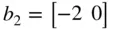
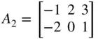
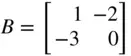
Suppose we have defined vectors a 1, a 2, b 1, b 2, and matrices A 1, A 2, B as follows:
>a1=[-1 2 3]; a2=[4 5 2]; b1=[1 -3]'; b2=[-2 0];  ,
,  ,
,  ,
,  >A1=[a1;a2], A2=[a1;[b2 1]], B=[b1 b2']
 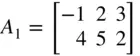 ,
,  ,
, 
Интервал:
Закладка:
Похожие книги на «Applied Numerical Methods Using MATLAB»
Представляем Вашему вниманию похожие книги на «Applied Numerical Methods Using MATLAB» списком для выбора. Мы отобрали схожую по названию и смыслу литературу в надежде предоставить читателям больше вариантов отыскать новые, интересные, ещё непрочитанные произведения.


Обсуждение, отзывы о книге «Applied Numerical Methods Using MATLAB» и просто собственные мнения читателей. Оставьте ваши комментарии, напишите, что Вы думаете о произведении, его смысле или главных героях. Укажите что конкретно понравилось, а что нет, и почему Вы так считаете.