Jane M. Horgan - Probability with R

and so on for x2, y2, x3, y3, x4, and y4. Then, for convenience, group the data into data frames as follows:

dataset1 <- data.frame(x1,y1) dataset2 <- data.frame(x2,y2) dataset3 <- data.frame(x3,y3) dataset4 <- data.frame(x4,y4)

When presented with data such as these, it is usual to obtain summary statistics. Let us do this using R .

To obtain the means of the variables in each data set, write

mean(dataset1) x1 y1 9.000000 7.500909 mean(dataset2) x2 y2 9.000000 7.497273 mean(dataset3) x3 y3 9.0 7.5 mean(dataset4) x4 y4 9.000000 7.500909

The means for the variables, as you can see, are practically identical as are the means for the variables.

Let us look at the standard deviations.

sd(dataset1) x1 y1 3.316625 2.031568 sd(dataset2) x2 y2 3.316625 2.028463 sd(dataset3) x3 y3 3.316625 2.030424 sd(dataset4) x4 y4 3.316625 2.030579

The standard deviations, as you can see, are also practically identical for the four variables, and also for the variables.

Calculating the mean and standard deviation is the usual way to summarize data. With these data, if this was all that we did, we would conclude naively that the four data sets are “equivalent,” since that is what the statistics say. But what do the statistics not say?

Investigating further, using graphical displays, gives a different picture. Pairwise plots would be the obvious exploratory technique to use with paired data.

par(mfrow = c(2, 2)) plot(x1,y1, xlim = c(0, 20), ylim = c(0, 13)) plot(x2,y2, xlim = c(0, 20), ylim = c(0, 13)) plot(x3,y3, xlim = c(0, 20), ylim = c(0, 13)) plot(x4,y4, xlim = c(0, 20), ylim = c(0, 13))

gives Fig. 3.20. Notice again the use of xlimand ylimto ensure that the scales on the axes are the same in the four plots, in order that a valid comparison can be made.

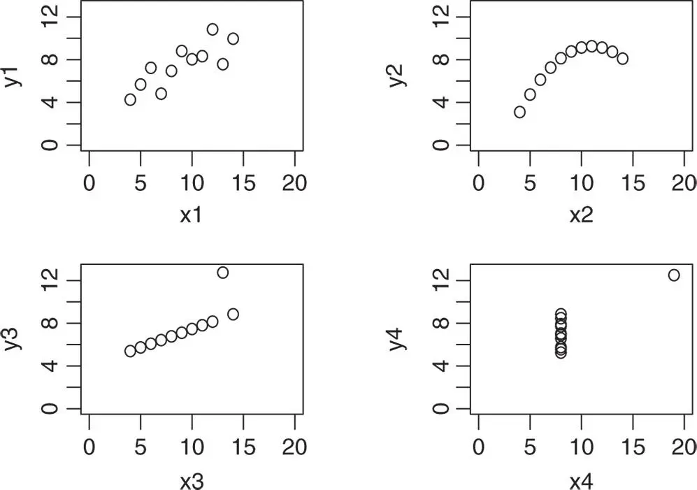
Figure 3.20Plots of Four Data Sets with Same Means and Standard Deviations

Examining Fig. 3.20, we see that there are very great differences in the data sets:

1 Data set 1 is linear with some scatter;

2 Data set 2 is quadratic;

3 Data set 3 has an outlier. If the outlier were removed the data would be linear;

4 Data set 4 contains values that are equal except for one outlier. If the outlier were removed, the data would be vertical.

Graphical displays are the core of getting “insight/feel” for the data. Such “insight/feel” does not come from the quantitative statistics; on the contrary, calculations of quantitative statistics should come after the exploratory data analysis using graphical displays.

1 Use the data in “results.txt” to develop boxplots of all the subjects on the same graph.

2 Obtain a stem and leaf of each subject in “results.txt.” Are there patterns emerging?

3 For the class of 50 students of computing detailed in Exercise 1.1, use R toform the stem‐and‐leaf display for each gender, and discuss the advantages of this representation compared to the traditional histogram;construct a box‐plot for each gender and discuss the findings.

4 Plot the marks in Architecture 1 against those in Architecture 2 and obtain the line of best fit. In your opinion, is it a suitable model for predicting the results obtained in Architecture 2 from those obtained in Architecture 1?

5 The following table gives the number of hours spent studying for the probability examination and the result obtained (%) by each of 10 students.Study hours548710610400Exam results73648070855086502025Plot the data and decide if there is a linear trend. If there is, use R to obtain the line of best fit.

6 The percentage of households with access to the Internet in Ireland in each of the years 2010–2017 is given in the following table:Year20102011201220132014201520162017Internet access7278818282858789This set of data is to be used as a training set to estimate Internet access in the future.Plot the data and decide if there is a linear trend.If there is, obtain the line of best fit.Can you predict what the Internet access will be in 2019?

1 In Appendix B, we show that the line of best fit is obtained whenandWrite a program in R to calculate and and use it to obtain the line that best fits the data in Exercise 5 above. Check your results using the lm(y˜x) function given in R.

2 When plotting in Fig. 3.10, we used font.main = 1 to ensure the main titles are in plain font.Alternative fonts available are2 = bold,3 = italic,4 = bold italic5 = symbol.Fonts may also be changed on the ‐ and ‐axis labels, with font.lab. Explore the effect of changing the fonts in Fig. 3.7.

1 Anscombe, F.J. (1973), Graphs in statistical analysis, American Statistician, 27, 1721.

2 Girolami, M. (2015), A First Course in Machine Learning, CRC Press.

Текст предоставлен ООО «ЛитРес».

Прочитайте эту книгу целиком, на ЛитРес.

Безопасно оплатить книгу можно банковской картой Visa, MasterCard, Maestro, со счета мобильного телефона, с платежного терминала, в салоне МТС или Связной, через PayPal, WebMoney, Яндекс.Деньги, QIWI Кошелек, бонусными картами или другим удобным Вам способом.