Jane M. Horgan - Probability with R

Write a program to calculate this, and apply it to the data in results.txt . Is it a reasonable approximation?

In addition to numerical summaries of statistical data, there are various pictorial representations and graphical displays available in R that have a more dramatic impact and make for a better understanding of the data. The ease and speed with which graphical displays can be produced is one of the important features of R . By writing

demo(graphics)

you will see examples of the many graphical procedures of R , along with the code needed to implement them. In this chapter, we will examine some of the most common of these.

A boxplot is a graphical summary based on the median, quartiles, and extreme values. To display the downtime data given in Example 1.1using a boxplot, write

boxplot(downtime)

which gives Fig. 3.1. Often called the Box and Whiskers Plot , the box represents the interquartile range that contains 50% of cases. The whiskers are the lines that extend from the box to the highest and lowest values. The line across the box indicates the median.

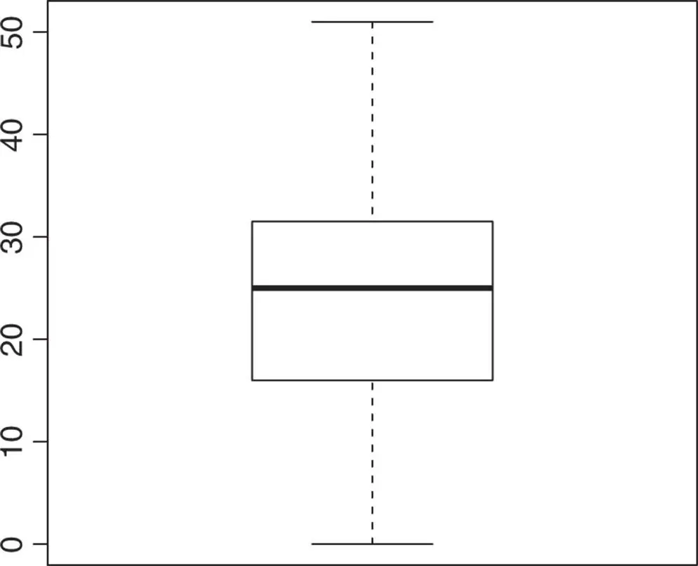
Figure 3.1A Simple Boxplot

To improve the look of the graph, we could label the axes as follows:

boxplot(downtime, xlab = "Downtime", ylab = "Minutes")

which gives Fig. 3.2.

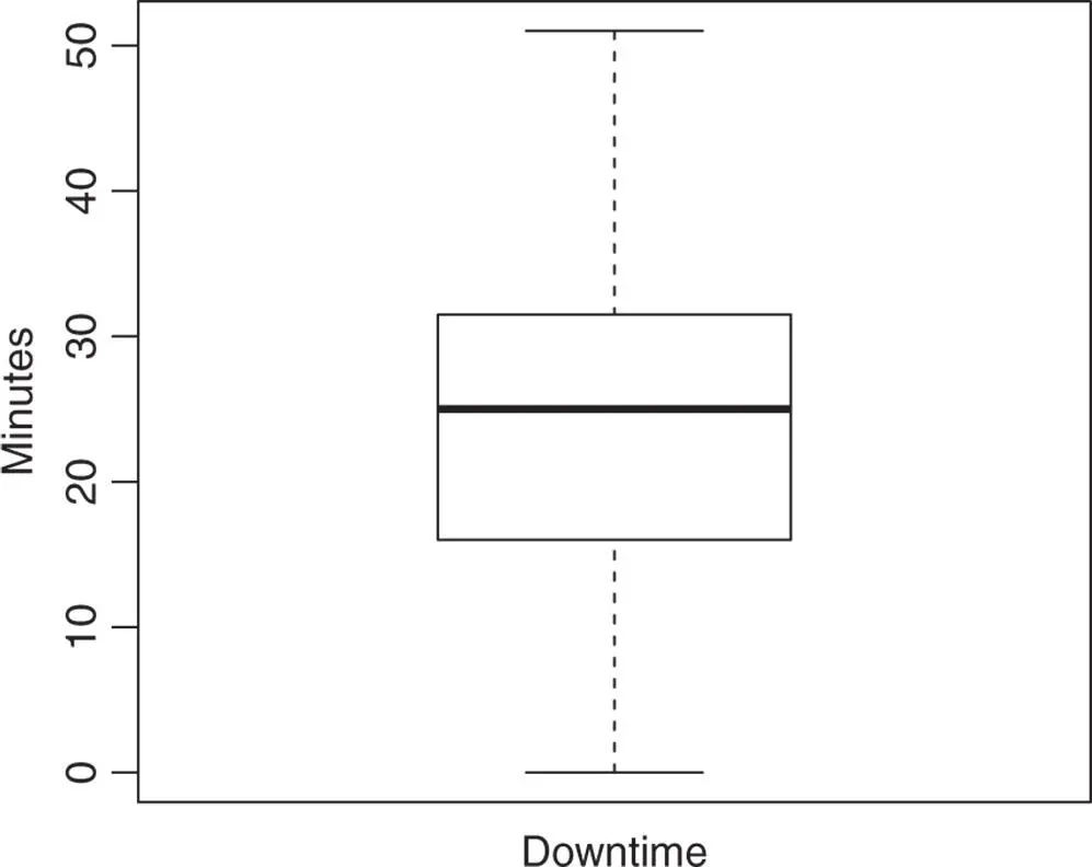
Figure 3.2A Boxplot with Axis Labels

Multiple boxplots can be displayed on the same axis, by adding extra arguments to the boxplot function. For example,

boxplot(results$arch1, results$arch2, xlab = "Architecture Semesters 1 and 2")

or simply

boxplot(arch1, arch2, xlab = "Architecture Semesters 1 and 2")

gives Fig. 3.3.

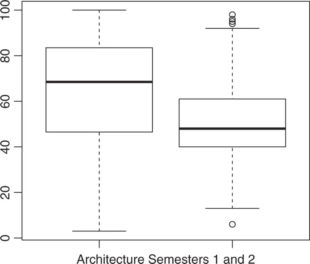
Figure 3.3Multiple Boxplots

Figure 3.3allows us to compare the performance of the students in Architecture in the two semesters. It shows, for example, that the marks are lower in Architecture in Semester 2 and the range of marks is narrower than those obtained in Architecture in Semester 1.

Notice also in Fig. 3.3that there are points outside the whiskers of the boxplot in Architecture in Semester 2. These points represent cases over 1.5 box lengths from the upper or lower end of the box and are called outliers . They are considered atypical of the data in general, being either extremely low or extremely high compared to the rest of the data.

Looking at Exercise 1.1 with the uncorrected data, Fig. 3.4is obtained using

boxplot(marks˜gendermarks)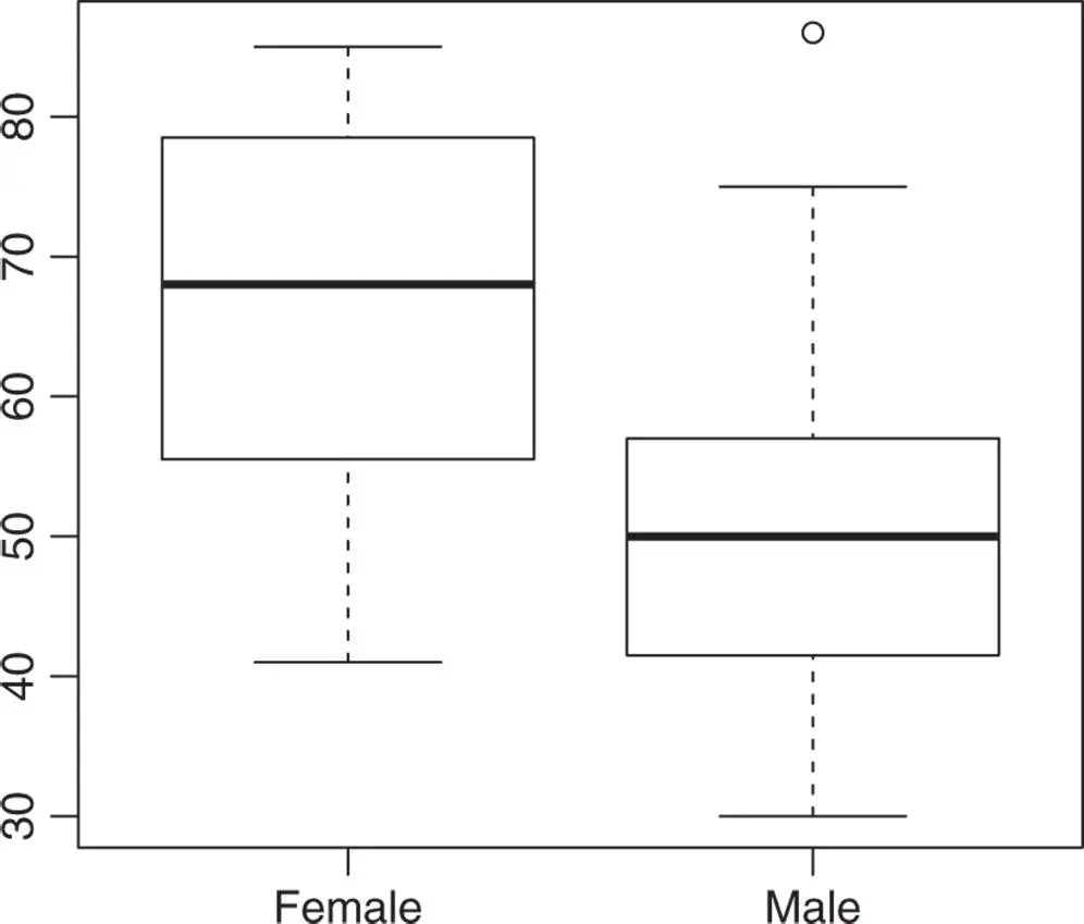

Figure 3.4A Gender Comparison

Notice the outlier in Fig. 3.4in the male boxplot, a value that appears large compared to the rest of the data. You will recall that a check on the examination results indicated that this value should have been 46, not 86, and we corrected it using

marks[34] <- 46

Repeating the analysis, after making this correction

boxplot(marks˜gendermarks)

gives Fig. 3.5.

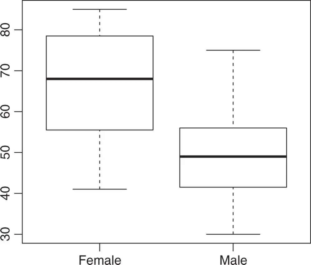
Figure 3.5A Gender Comparison (corrected)

You will now observe from Fig. 3.5that there are no outliers in the male or female data. In this way, a boxplot may be used as a data validation tool. Of course, it is possible that the mark of 86 may in fact be valid, and that a male student did indeed obtain a mark that was much higher than his classmates. A boxplot highlights this and alerts us to the possibility of an error.

To compare the performance of females and males in Architecture in Semester 1, write

gender <- factor(gender, levels = c("f", "m"), labels = c("Female", "Male"))

which changes the labels from “f ” and “m” to “Female” and “Male,” respectively. Then

boxplot(arch1∼gender, ylab = "Marks (%)", main = "Architecture Semester 1", font.main = 1)

outputs Fig. 3.6.

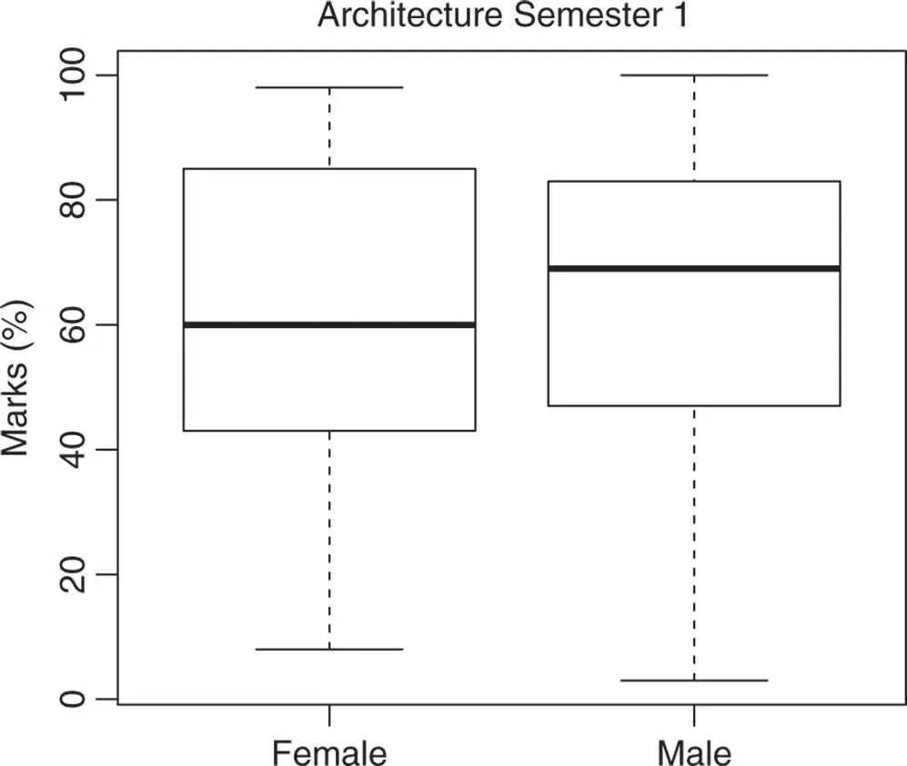
Figure 3.6A Gender Comparison

Notice the effect of using main = "Architecture Semester 1"that puts the title on the diagram. Also, the use of font.main = 1ensures that the main title is in plain font.

We can display plots as a matrix using the parfunction: par(mfrow = c(2,2))causes the outputs to be displayed in a array.

par(mfrow = c(2,2)) boxplot(arch1∼gender, main = "Architecture Semester 1", font.main = 1) boxplot(arch2∼gender, main = "Architecture Semester 2", font.main = 1) boxplot(prog1∼gender, main = "Programming Semester 1", font.main = 1) boxplot(prog2∼gender, main = "Programming Semester 2", font.main = 1)

produces Fig. 3.7.

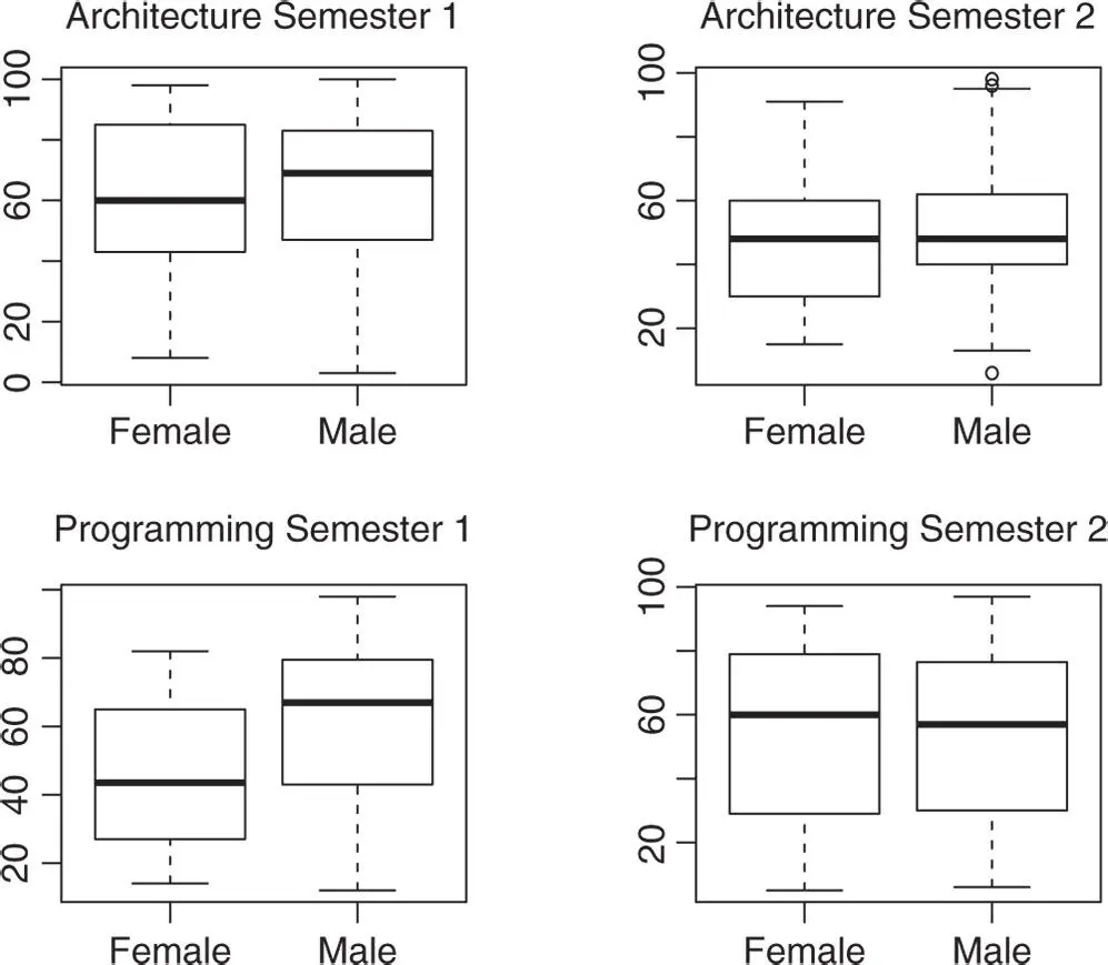
Figure 3.7A Lattice of Boxplots

We see from Fig. 3.7that female students seem to do less well than their male counterparts in Programming in Semester 1, where the median mark of the females is considerably lower than that of the males: it is lower even than the first quartile of the male marks. In the other subjects, there do not appear to be any substantial differences.

To undo a matrix‐type output, write

par(mfrow = c(1,1))

which restores the graphics output to the full screen.

A histogram is a graphical display of frequencies in categories of a variable and is the traditional way of examining the “shape” of the data.

hist(prog1, xlab ="Marks (%)", main = "Programming Semester 1")

yields Fig. 3.8.

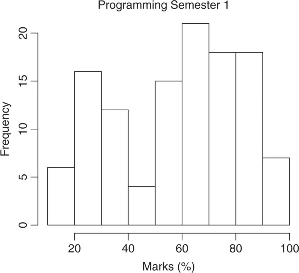
Figure 3.8A Histogram with Default Breaks

As we can see from Fig. 3.8, histgives the count of the observations that fall within the categories or “bins” as they are sometimes called. R chooses a “suitable” number of categories, unless otherwise specified. Alternatively, breaksmay be used as an argument in histto determine the number of categories. For example, to get five categories of equal width, you need to include breaks = 5as an argument.

hist(prog1, xlab = "Marks (%)", main = "Programming Semester 1", breaks = 5)