Jane M. Horgan - Probability with R
Здесь есть возможность читать онлайн «Jane M. Horgan - Probability with R» — ознакомительный отрывок электронной книги совершенно бесплатно, а после прочтения отрывка купить полную версию. В некоторых случаях можно слушать аудио, скачать через торрент в формате fb2 и присутствует краткое содержание. Жанр: unrecognised, на английском языке. Описание произведения, (предисловие) а так же отзывы посетителей доступны на портале библиотеки ЛибКат.

- Название:Probability with R
- Автор:
- Жанр:
- Год:неизвестен
- ISBN:нет данных
- Рейтинг книги:3 / 5. Голосов: 1
-
Избранное:Добавить в избранное
- Отзывы:
-
Ваша оценка:
Probability with R: краткое содержание, описание и аннотация
Предлагаем к чтению аннотацию, описание, краткое содержание или предисловие (зависит от того, что написал сам автор книги «Probability with R»). Если вы не нашли необходимую информацию о книге — напишите в комментариях, мы постараемся отыскать её.
is used throughout the text, not only as a tool for calculation and data analysis, but also to illustrate concepts of probability and to simulate distributions. The examples in
cover a wide range of computer science applications, including: testing program performance; measuring response time and CPU time; estimating the reliability of components and systems; evaluating algorithms and queuing systems.
Chapters cover: The R language; summarizing statistical data; graphical displays; the fundamentals of probability; reliability; discrete and continuous distributions; and more.
This second edition includes:
improved R code throughout the text, as well as new procedures, packages and interfaces; updated and additional examples, exercises and projects covering recent developments of computing; an introduction to bivariate discrete distributions together with the R functions used to handle large matrices of conditional probabilities, which are often needed in machine translation; an introduction to linear regression with particular emphasis on its application to machine learning using testing and training data; a new section on spam filtering using Bayes theorem to develop the filters; an extended range of Poisson applications such as network failures, website hits, virus attacks and accessing the cloud; use of new allocation functions in R to deal with hash table collision, server overload and the general allocation problem. The book is supplemented with a Wiley Book Companion Site featuring data and solutions to exercises within the book.
Primarily addressed to students of computer science and related areas,
is also an excellent text for students of engineering and the general sciences. Computing professionals who need to understand the relevance of probability in their areas of practice will find it useful.
Probability with R — читать онлайн ознакомительный отрывок
Ниже представлен текст книги, разбитый по страницам. Система сохранения места последней прочитанной страницы, позволяет с удобством читать онлайн бесплатно книгу «Probability with R», без необходимости каждый раз заново искать на чём Вы остановились. Поставьте закладку, и сможете в любой момент перейти на страницу, на которой закончили чтение.
Интервал:
Закладка:
| Observation Numbers | 1 | 2 | 3 | 4 | 5 | 6 | 7 | 8 | 9 | 10 |
 |
8.5 | 9.4 | 5.4 | 11.7 | 6.5 | 10.3 | 12.7 | 11.0 | 15.4 | 2.8 |
 |
49.4 | 43.0 | 19.3 | 56.4 | 28.3 | 53.7 | 58.1 | 28.7 | 80.7 | 13.6 |
Use the training set to obtain the line of best fit of  on
on  and the testing set to examine how well the line fits the data.
First, read the training set 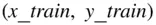 into R .
x_train <- c(11.8, 10.8, 8.6, ..., 8.9) y_train <- c(31.3, 59.9, 27.6, ..., 38.5)
and the testing set 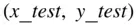
x_test <- c(8.5, 9.4, 5.4, …, 2.8) y_test <- c(49.4, 43.0, 19.3,…, 13.6)
Then, plot the training set, to establish if a linear trend exists.
plot(x_train, y_train, main = "Training Data", font.main = 1)
gives Fig. 3.17.
Figure 3.17The Scatter of the Training Data
Since Fig. 3.17shows a linear trend, we obtain the line of best fit of  on
on  , and superimpose it on the scatter diagram in Fig. 3.17. In R , write
abline(lm(y_train ∼ x_train))
to get Fig. 3.18.
Figure 3.18The Line of Best Fit for the Training Data
Next, we use the testing data to decide on the suitability of the line.
The coefficients of the line are obtained in R with
lm(formula = y_train ∼ x_train) Coefficients: (Intercept) x_train -0.9764 4.9959
The estimated values  are calculated in R as follows:
y_est <- - 0.9764 + 4.9959 * x_test round(y_est, 1)
which gives
y_est 41.5 46.0 26.0 57.5 31.5 50.5 62.5 54.0 76.0 13.0
We now compare these estimated values with the observed values.
y_test 49.4 43.0 19.3 56.4 28.7 53.7 58.1 54.0 80.7 13.6plot(x_test, y_test, main = "Testing Data", font.main = 1) abline(lm(y_train ∼ x_train)) # plot the line of best fit segments(x_test, y_test, x_test, y_est)
gives Fig. 3.19. Here, segmentsplots vertical lines between (x_test, y_test) and (x_test, y-est)
Figure 3.19shows the observed values,  , along with the values estimated from the line,
  . The vertical lines illustrate the differences between them. A decision has to be made then as to whether or not the line is a “good fit” or whether an alternative model should be investigated.
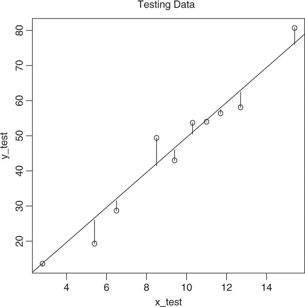
Figure 3.19Differences Between Observed and Estimated  Values in the Testing Set
The line of best fit is the simplest regression model; it uses just one independent variable for prediction. In real‐life situations, many more independent variables or other models, such as, for example a quadratic, may be required, but for supervised learning, the approach is always the same:
Determine if there is a relationship between the dependent variable and the independent variables;
Fit the model to the training data;
Test the suitability of the model by predicting the ‐values in the testing data from the model and by comparing the observed and predicted ‐values.
The predictions from these models assumes that the trend, based on the data analyzed, continues to exist. Should the trend change, for example, when a house pricing model is estimated from data before an economic crash, the predictions will not be valid.
Regression analysis is just one of the many techniques from the area of Probability and Statistics that machine learning invokes. We will encounter more in later chapters. Should you wish to go into this topic more deeply, we recommend the book, A First Course in Machine Learning by Girolami (2015).
3.7 GRAPHICAL DISPLAYS VERSUS SUMMARY STATISTICS
Before we finish, let us look at a simple, classic example of the importance of using graphical displays to provide insight into the data. The example is that of Anscombe (1973), who provides four data sets, given in Table 3.3and often referred to as the Anscombe Quartet . Each data set consists of two variables on which there are 11 observations.
TABLE 3.3The Anscombe Quartet
| Data Set 1 | Data Set 2 | Data Set 3 | Data Set 4 | ||||
| x1 | y1 | x2 | y2 | x3 | y3 | x4 | y4 |
| 10 | 8.04 | 10 | 9.14 | 10 | 7.46 | 8 | 6.58 |
| 8 | 6.95 | 8 | 8.14 | 8 | 6.77 | 8 | 5.76 |
| 13 | 7.58 | 13 | 8.74 | 13 | 12.74 | 8 | 7.71 |
| 9 | 8.81 | 9 | 8.77 | 9 | 7.11 | 8 | 8.84 |
| 11 | 8.33 | 11 | 9.26 | 11 | 7.81 | 8 | 8.47 |
| 14 | 9.96 | 14 | 8.10 | 14 | 8.84 | 8 | 7.04 |
| 6 | 7.24 | 6 | 6.13 | 6 | 6.08 | 8 | 5.25 |
| 4 | 4.26 | 4 | 3.10 | 4 | 5.39 | 19 | 12.50 |
| 12 | 10.84 | 12 | 9.13 | 12 | 8.15 | 8 | 5.56 |
| 7 | 4.82 | 7 | 7.26 | 7 | 6.42 | 8 | 7.91 |
| 5 | 5.68 | 5 | 4.74 | 5 | 5.73 | 8 | 6.89 |
First, read the data into separate vectors.
x1 <- c(10, 8, 13, 9, 11, 14, 6, 4, 12, 7, 5) y1 <- c(8.04, 6.95, 7.58, 8.81, 8.33, 9.96, 7.24, 4.26, 10.84, 4.82, 5.68)
Читать дальшеИнтервал:
Закладка:
Похожие книги на «Probability with R»
Представляем Вашему вниманию похожие книги на «Probability with R» списком для выбора. Мы отобрали схожую по названию и смыслу литературу в надежде предоставить читателям больше вариантов отыскать новые, интересные, ещё непрочитанные произведения.


Обсуждение, отзывы о книге «Probability with R» и просто собственные мнения читателей. Оставьте ваши комментарии, напишите, что Вы думаете о произведении, его смысле или главных героях. Укажите что конкретно понравилось, а что нет, и почему Вы так считаете.