Jane M. Horgan - Probability with R

gives Fig. 3.9

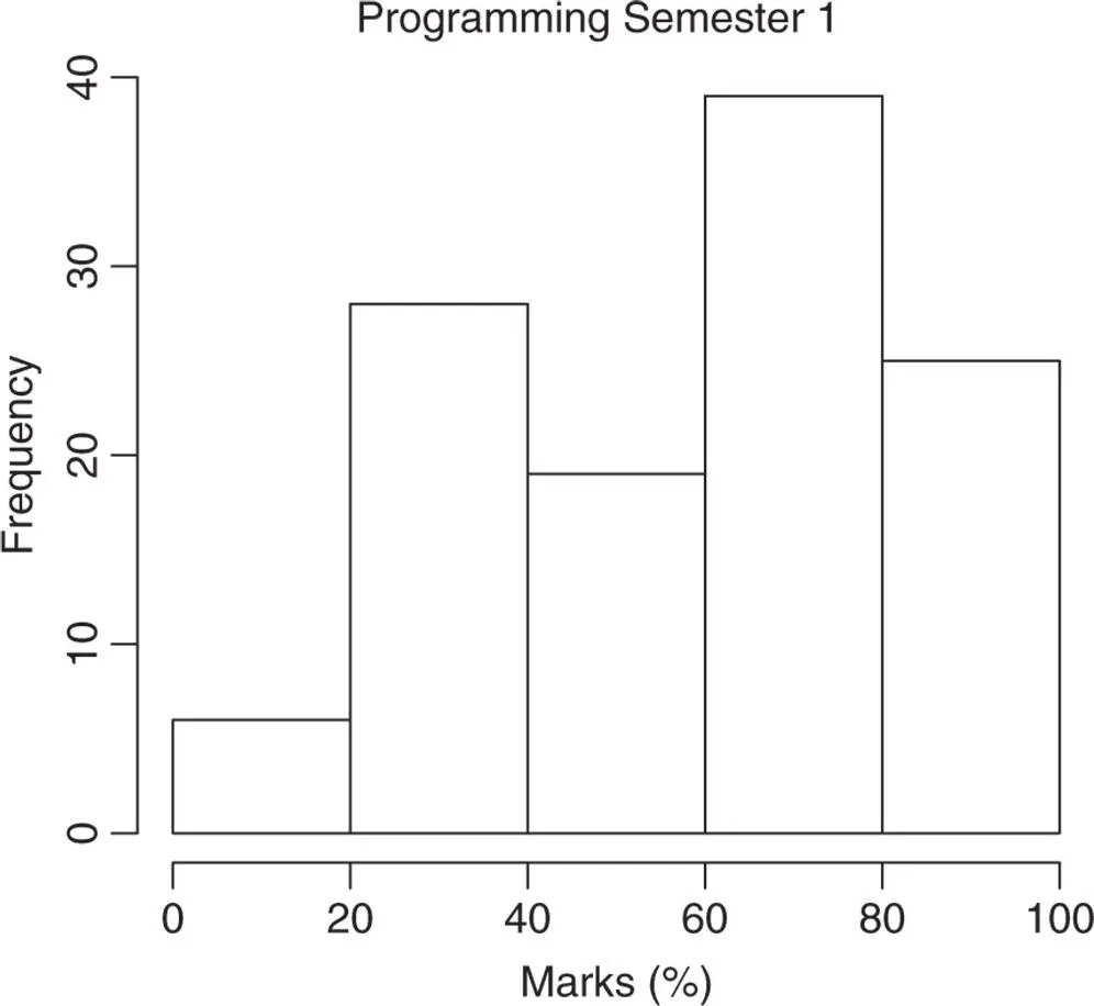
Figure 3.9A Histogram with Five Breaks of Equal Width

Recall that parcan be used to represent all the subjects in one diagram. Type

par (mfrow = c(2,2)) hist(arch1, xlab = "Architecture", main = "Semester 1", ylim = c(0, 35)) hist(arch2, xlab = "Architecture", main = "Semester 2", ylim = c(0, 35)) hist(prog1, xlab = "Programming", main = " ", ylim = c(0, 35)) hist(prog2, xlab = "Programming", main = " ", ylim = c(0, 35))

to get Fig. 3.10. The ylim = c(0, 35)ensures that the ‐axis is the same scale for all the four subjects.

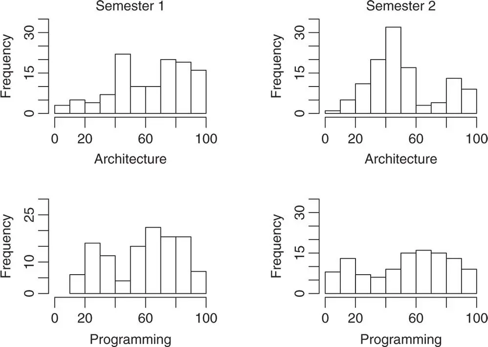
Figure 3.10Histogram of Each Subject in Each Semester

Up until now, we have invoked the default parameters of the histogram, notably the bin widths are equal and the frequency in each bin is calculated. These parameters may be changed as appropriate. For example, you may want to specify the bin break‐points to represent the failures and the various classes of passes and honors.

bins <- c(0, 40, 60, 80, 100)hist(prog1, xlab ="Marks (%)", main = "Programming Semester 1", breaks = bins)

yields Fig. 3.11.

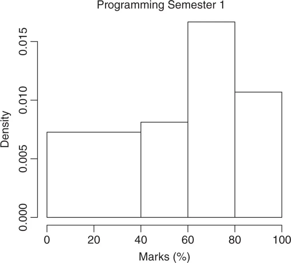
Figure 3.11A Histogram with Breaks of a Specified Width

In Fig. 3.11, observe that the ‐axis now represents the density. When the bins are not of equal length, R returns a normalized histogram, so that its total area is equal to one.

To get a histogram of percentages, write in R

h <- hist(prog1, plot = FALSE, breaks = 5) #this postpones the plot display h$density <- h$counts/sum(h$counts)*100 #this calculates percentages plot(h, xlab = "Marks (%)", freq = FALSE, ylab = "Percentage", main = "Programming Semester 1")

The output is given in Fig. 3.12. The # allows for a comment. Anything written after # is ignored.

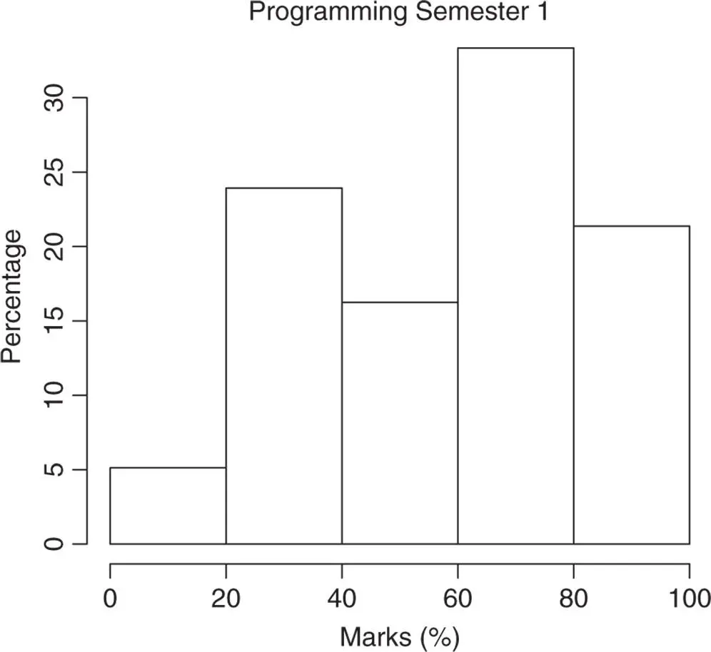
Figure 3.12Histogram with Percentages

The stem and leaf diagram is a more modern way of displaying data than the histogram. It is a depiction of the shape of the data using the actual numbers observed. Similar to the histogram, the stem and leaf gives the frequencies of categories of the variable, but it goes further than that and gives the actual values in each category.

The marks obtained in Programming in Semester 1 are depicted as a stem and leaf diagram using

stem(prog1)

which yields Fig. 3.13.

The decimal point is 1 digit(s) to the right of the | 1 | 2344 1 | 59 2 | 11 2 | 5556777889999 3 | 0113 3 | 6 4 | 00000000 4 | 6779 5 | 12223344 5 | 56679 6 | 0011123444 6 | 566777888999 7 | 0112344 7 | 5666666899 8 | 001112222334 8 | 5678899 9 | 0122 9 | 7778

FIGURE 3.13A Stem and Leaf Diagram

From Fig. 3.13, we are able to see the individual observations, as well as the shape of the data as a whole. Notice that there are many marks of exactly 40, whereas just one student obtains a mark between 35 and 40. One wonders if this has anything to do with the fact that 40 is a pass, and that the examiner has been generous to borderline students. This point would go unnoticed with a histogram.

Plots of data are useful to investigate relationships between variables. To examine, for example, the relationship between the performance of students in Programming in Semesters 1 and 2, we could write

plot(prog1, prog2, xlab = "Programming Semester 1", ylab = "Programming Semester 2")

to obtain Fig. 3.14.

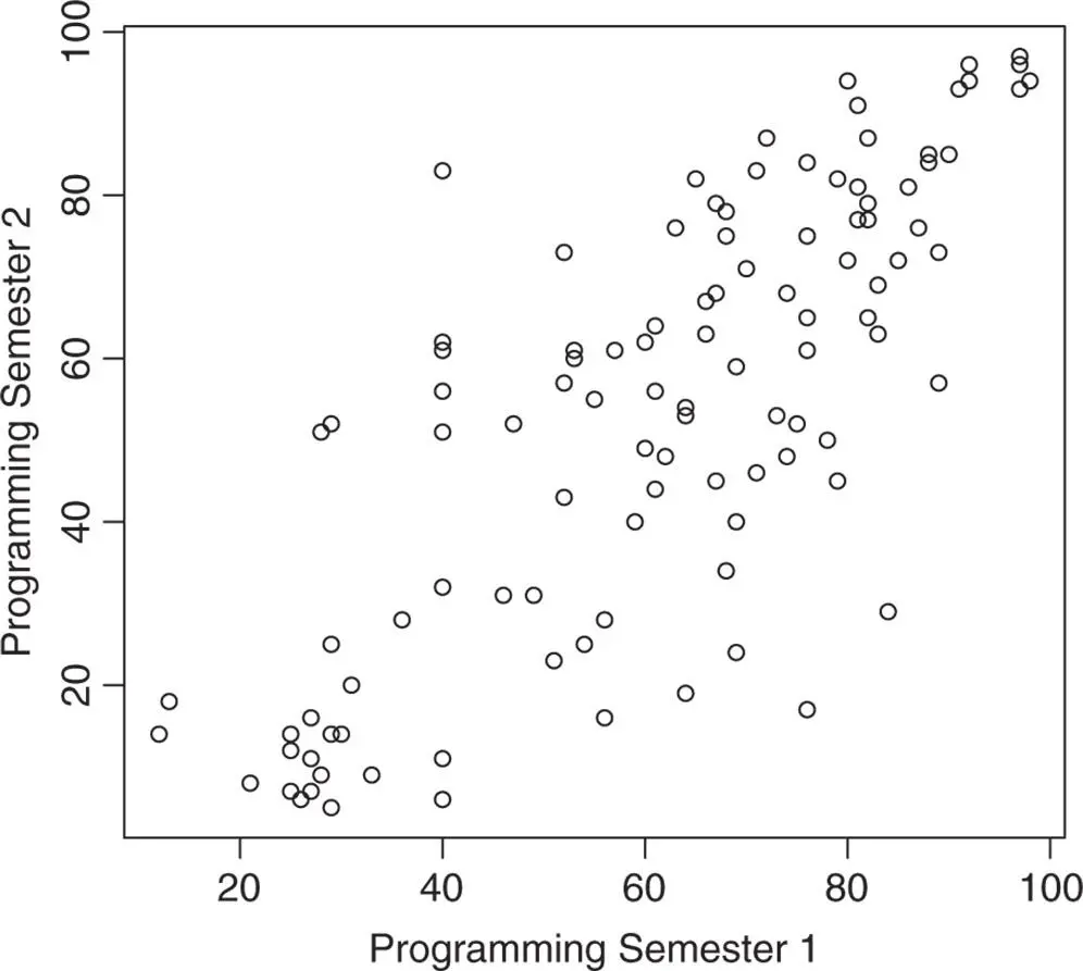
Figure 3.14A Scatter Plot

When more than two variables are involved, R provides a facility for producing scatter plots of all possible pairs.

To do this, first create a data frame of all the variables that you want to compare.

courses <- results[2:5]

This creates a data frame containing the second to the fifth variables in , that is, and . Writing

pairs(courses)

or equivalently

pairs(results[2:5])

will generate Fig. 3.15, which, as you can see, gives scatter plots for all possible pairs.

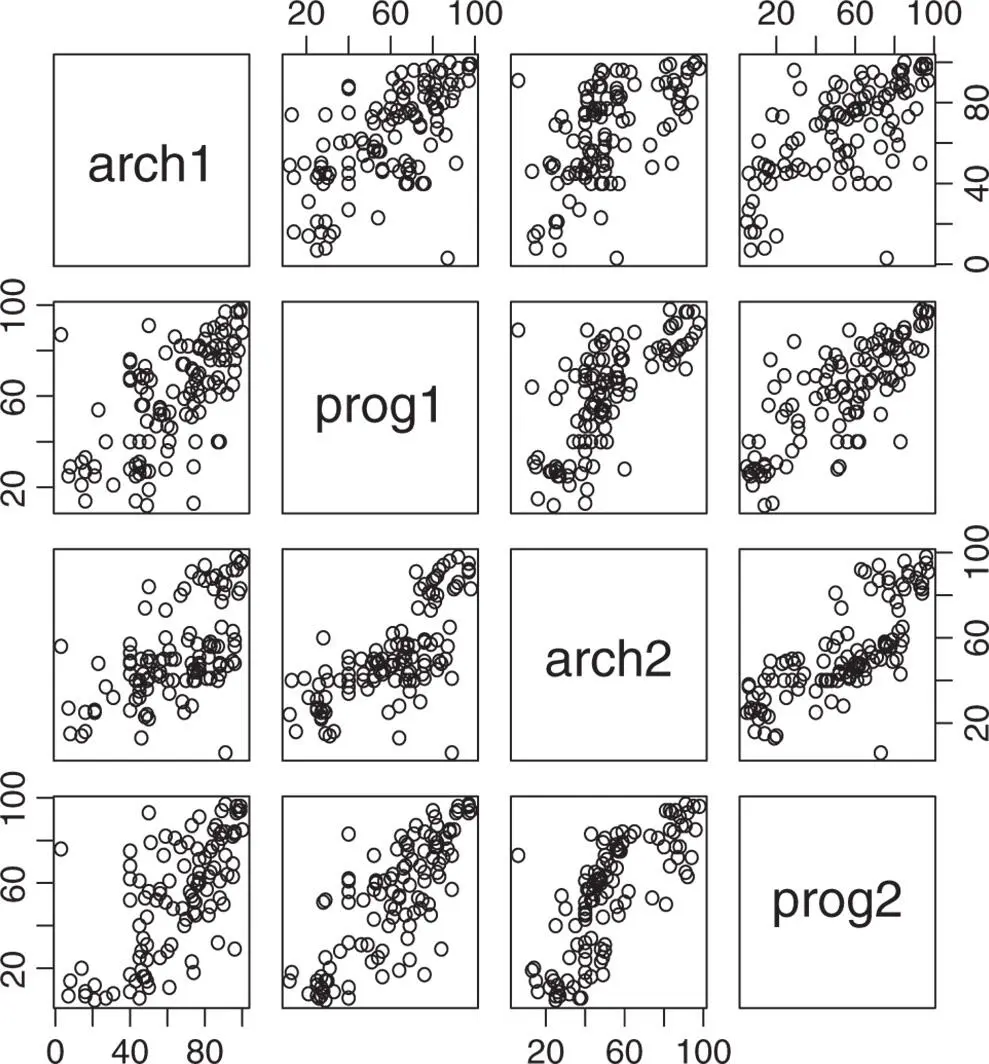
Figure 3.15Use of the Function

Returning to Fig. 3.14, we can see that there is a in these data. One variable increases with the other; not surprisingly, students doing well in Programming in Semester 1 are likely to do well also in Programming in Semester 2, and those doing badly in Semester 1 will tend to do badly in Semester 2. We might ask, if it is possible to estimate the Semester 2 results from those obtained in Semester 1.

In the case of the Programming subjects, we have a set of points ( , ), and having established, from the scatter plot, that a linear trend exists, we attempt to fit a line that best fits the data. In R

lm(prog2∼prog1)

calculates what is referred to as the linear model (lm) of on , or simply the line