Jane M. Horgan - Probability with R

First, subtract the mean from each data point.

downtime - meandown [1] -25.04347826 -24.04347826 -23.04347826 -13.04347826 -13.04347826 [6] -11.04347826 -7.04347826 -4.04347826 -4.04347826 -2.04347826 [11] -1.04347826 -0.04347826 3.95652174 2.95652174 4.95652174 [16] 4.95652174 4.95652174 7.95652174 10.95652174 18.95652174 [21] 19.95652174 21.95652174 25.95652174

Then, obtain the squares of these differences.

(downtime - meandown)^2 [1] 6.271758e+02 5.780888e+02 5.310019e+02 1.701323e+02 1.701323e+02 [6] 1.219584e+02 4.961059e+01 1.634972e+01 1.634972e+01 4.175803e+00 [11] 1.088847e+00 1.890359e-03 1.565406e+01 8.741021e+00 2.456711e+01 [16] 2.456711e+01 2.456711e+01 6.330624e+01 1.200454e+02 3.593497e+02 [21] 3.982628e+02 4.820888e+02 6.737410e+02

Sum the squared differences.

sum((downtime - meandown)^2) [1] 4480.957

Finally, divide this sum by length(downtime)‐1and take the square root.

sqrt(sum((downtime -meandown)^2)/(length(downtime)-1)) [1] 14.27164

You will recall that R has built‐in functions to calculate the most commonly used statistical measures. You will also recall that the mean and the standard deviation can be obtained directly with

mean(downtime) [1] 25.04348 sd(downtime) [1] 14.27164

We took you through the calculations to illustrate how easy it is to program in R .

Occasionally, you might require some statistical functions that are not available in R . You will need to create your own function. Let us take, as an example, the skewness coefficient, which measures how much the data differ from symmetry.

The skewness coefficient is defined as

(2.1)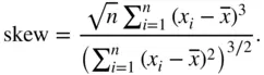

A perfectly symmetrical set of data will have a skewness of 0; when the skewness coefficient is substantially greater than 0, the data are positively asymmetric with a long tail to the right, and a negative skewness coefficient means that data are negatively asymmetric with a long tail to the left. As a rule of thumb, if the skewness is outside the interval , the data are considered to be highly skewed. If it is between 1 and 0.5 or 0.5 and 1, the data are moderately skewed.

The following syntax calculates the skewness coefficient of a set of data and assigns it to a function called that has one argument .

skew <- function(x) { xbar <- mean(x) sum2 <- sum((x-xbar)^2, na.rm = T) sum3 <- sum((x-xbar)^3, na.rm = T) skew <- (sqrt(length(x))* sum3)/(sum2^(1.5)) skew}

You will agree that the conventions of vector calculations make it very easy to calculate statistical functions.

When skew has been defined, you can calculate the skewness on any data set. For example,

skew(downtime)

gives

[1] -0.04818095

which indicates that the data is slightly negatively skewed.

Looking again at the data given Example 2.1, let us calculate the skewness coefficient

skew(usage) [1] 1.322147

which illustrates that the data is highly skewed. Recall that the first two values are outliers in the sense that they are very much larger than the other values in the data set. If we calculate the skewness with those values removed, we get

skew(usage[3:9]) [1] 0.4651059

which is very much smaller than that obtained with the full set.

There are various ways of developing programs in R .

The most useful way of writing programs is by means of R 's own built‐in editor called . From at the toolbar click on New Script ( File/New Script ). You are then presented with a blank screen to develop your program. When done, you may save and retrieve this program as you wish. File/Save causes the file to be saved. You may designate the name you want to call it, and it will be given a .R extension. In subsequent sessions, File/Open Script brings up all the .R files that you have saved. You can select the one you wish to use.

When you want to execute a line or group of lines, highlight them and press Ctrl/R , that is, Ctrl and the letter R simultaneously. The commands are then transferred to the control window and executed.

Alternatively, if the program is short, it may be developed interactively while working at your computer.

Programs may also be developed in a text editor, like Notepad, saved with the . R extension and retrieved using the sourcestatement.

source("C:\\test")

retrieves the program named test.R from the C directory. Another way of doing this, while working in R , is to click on on the tool bar where you will be given the option to Source R code , and then you can browse and retrieve the program you require.

1 For the class of 50 students of computing detailed in Exercise 1.1, use R to:obtain the summary statistics for each gender, and for the entire class;calculate the deciles for each gender and for the entire class;obtain the skewness coefficient for the females and for the males.

2 It is required to estimate the number of message buffers in use in the main memory of the computer system at Power Products Ltd. To do this, 20 programs were run, and the number of message buffers in use were found to beCalculate the average number of buffers used. What is the standard deviation? Would you say these data are skewed?

3 To get an idea of the runtime of a particular server, 20 jobs were processed and their execution times (in seconds) were observed as follows:Examine these data and calculate appropriate measures of central tendency and dispersion.

4 Ten data sets were used to run a program and measure the execution time. The results (in milliseconds) were observed as follows:Use appropriate measures of central tendency and dispersion to describe these data.

5 The following data give the amount of time (in minutes) in one day spent on Facebook by each of 15 students.Obtain appropriate measures of central tendency and measures of dispersion for these data.

Write the skewness program, and use it to calculate the skewness coefficient of the four examination subjects in results.txt . What can you say about these data?

Pearson has given an approximate formula for the skewness that is easier to calculate than the exact formula given in Equation 2.1.