Donald W. McRobbie - Essentials of MRI Safety
Здесь есть возможность читать онлайн «Donald W. McRobbie - Essentials of MRI Safety» — ознакомительный отрывок электронной книги совершенно бесплатно, а после прочтения отрывка купить полную версию. В некоторых случаях можно слушать аудио, скачать через торрент в формате fb2 и присутствует краткое содержание. Жанр: unrecognised, на английском языке. Описание произведения, (предисловие) а так же отзывы посетителей доступны на портале библиотеки ЛибКат.
- Название:Essentials of MRI Safety
- Автор:
- Жанр:
- Год:неизвестен
- ISBN:нет данных
- Рейтинг книги:4 / 5. Голосов: 1
-
Избранное:Добавить в избранное
- Отзывы:
-
Ваша оценка:
Essentials of MRI Safety: краткое содержание, описание и аннотация
Предлагаем к чтению аннотацию, описание, краткое содержание или предисловие (зависит от того, что написал сам автор книги «Essentials of MRI Safety»). Если вы не нашли необходимую информацию о книге — напишите в комментариях, мы постараемся отыскать её.
Reflects the most current research, guidelines, and MRI safety information Explains procedures for scanning pregnant women, managing MRI noise exposure, and handling emergency situations Prepares candidates for the American Board of MR Safety exam and other professional certifications Aligns with MRI safety roles such as MR Medical Director (MRMD), MR Safety Officer (MRSO) and MR Safety Expert (MRSE) Contains numerous illustrations, figures, self-assessment tests, key references, and extensive appendices
is an indispensable text for all radiographers and radiologists, as well as physicists, engineers, and researchers with an interest in MRI.
Essentials of MRI Safety — читать онлайн ознакомительный отрывок
Ниже представлен текст книги, разбитый по страницам. Система сохранения места последней прочитанной страницы, позволяет с удобством читать онлайн бесплатно книгу «Essentials of MRI Safety», без необходимости каждый раз заново искать на чём Вы остановились. Поставьте закладку, и сможете в любой момент перейти на страницу, на которой закончили чтение.
Интервал:
Закладка:
So, what is magnetic field strength in actuality? It is given the symbol Hand has units of amperes per meter (A m −1). It is defined in terms of a cylindrical electromagnet, just like our scanner – the current in the windings generates an H‐field. In free space
(1.5) 
μ 0is the magnetic permeability in a vacuum, equal to 4π x10 −7henrys per meter (H m −1).
One way of visualizing magnetic fields is through magnetic field lines. If you have ever done the experiment of introducing iron filings to the proximity of a simple bar magnet you may have observed the pattern shown in Figure 1.23a. These illustrate the magnetic “lines of force”. A small compass needle positioned anywhere will align with these. We can think of the magnetic flux density as being the intensity of grouping of these lines: the more closely grouped together, the stronger the B‐field.
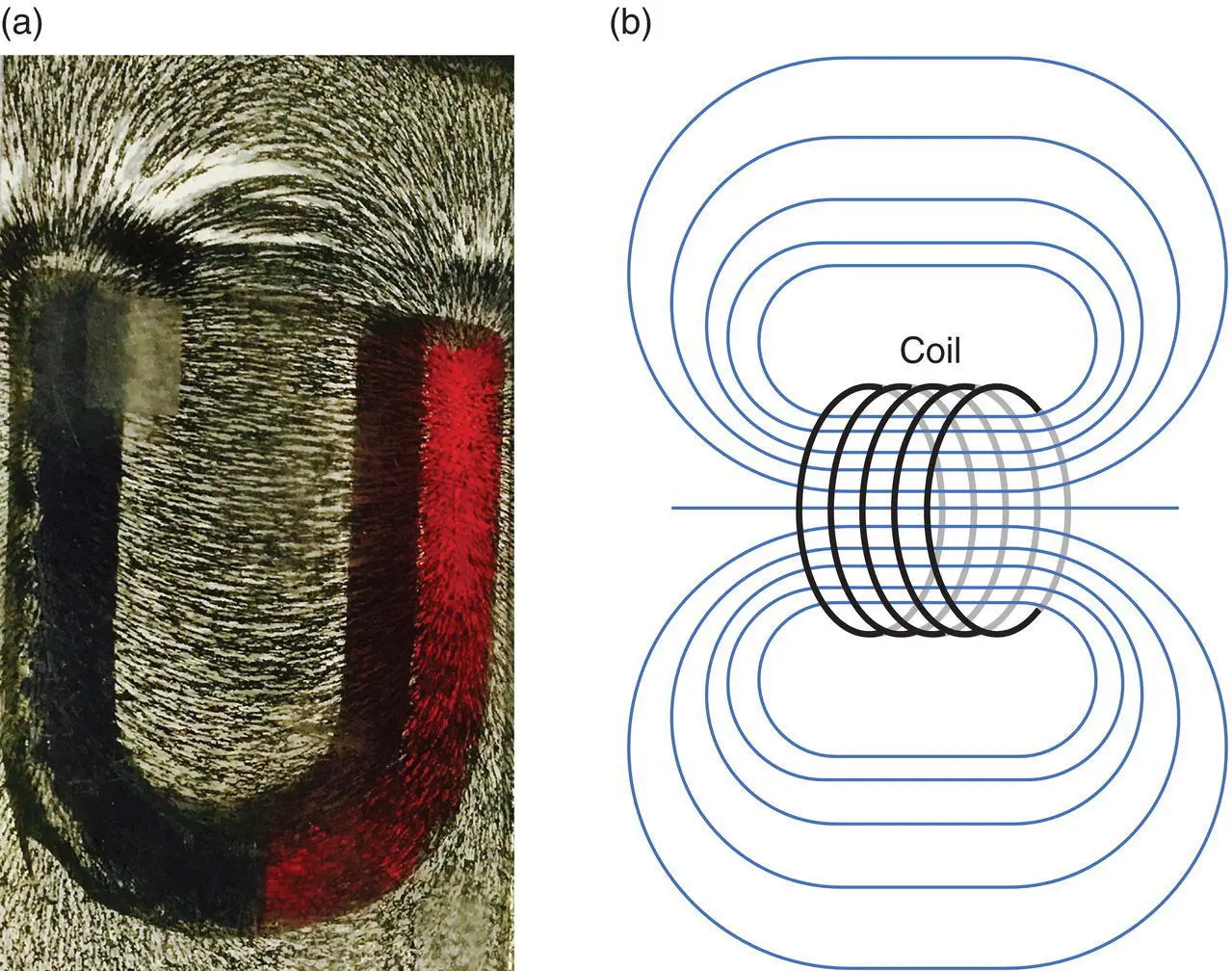
Figure 1.23 Magnetic field lines of force: (a) seen in the pattern of iron filings around a permanent magnet; (b) from an electromagnet.
B0 fringe field
The most uniform and dense grouping of lines of force for an MR magnet ( Figure 1.23b) occurs within the bore. As we move away from the bore the lines diverge and consequently the B‐field decreases. We call this region the fringe field . Your scanner manufacturer provides field maps showing fringe field contours at 0.5, 1, 3, 5, 10, 20, 40, and 200 mT [4] ( Figure 1.24). These are important for MRI suite design ( Chapter 12). A modern MRI system utilizes self‐shielding in order to reduce the spatial extent of the fringe field ( Figure 1.25).
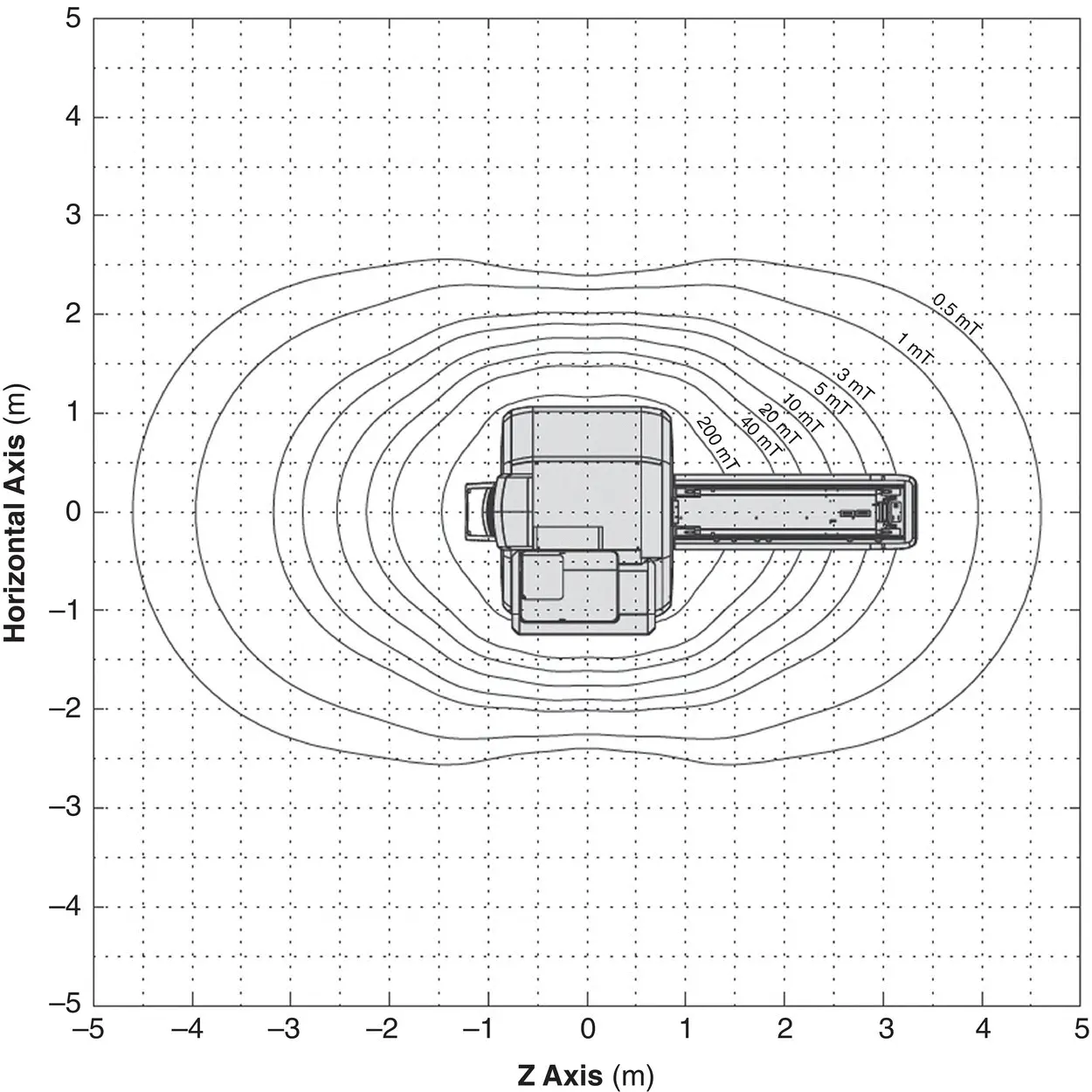
Figure 1.24 Fringe field contours at 0.5, 1, 3, 5, 10, 20, 40 and 200 mT for a 3 T MR magnet. Reproduced with permission of Siemens Healthineers.
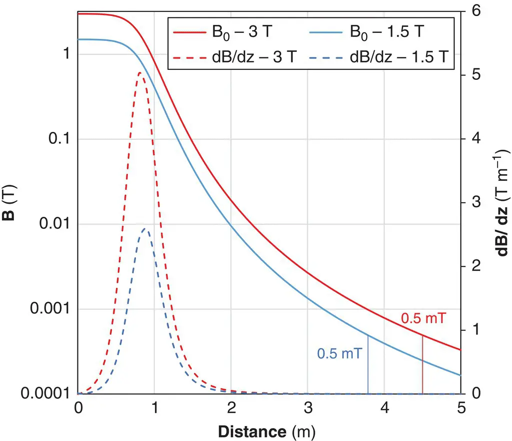
Figure 1.25 The magnitude of the B 0fringe field (solid lines, logarithmic LH scale) and its spatial gradient dB/dz (dashed lines, linear RH scale) along the z‐axis simulated for shielded 1.5 and 3 T MRI magnets. The vertical lines indicate the locations of the 0.5 mT contour. The iso‐centre is located at z=0, and the bore entrance at 0.8 m.
Fringe field spatial gradient
As we move further from the bore of the magnet, the lines of force diverge, and the fringe field decreases ( Figure 1.23b). The amount it decreases with distance is known as the fringe field spatial gradient , specified in T m −1. The fringe field spatial gradient is responsible for the attractive force on ferromagnetic objects. Your manufacturer is required to provide you with information about the fringe field gradient. Figure 1.25shows how the B 0field and its spatial gradient dB/dz vary along the z‐axis. The fringe field is compressed for the shielded magnet but produces a stronger spatial gradient close to the bore entrance. This is highly significant for projectile safety.
MYTHBUSTER:
The fringe spatial field gradient is always present as long as the main static B 0field exists. It should not be confused with the imaging gradients.
The imaging gradients
Gradient amplitude is measured in mT m −1(milli‐tesla per meter). When a gradient pulse is applied, e.g. along the x‐axis, the total B experienced at a point x is
(1.6) 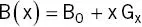
Example 1.3 B zfrom a gradient
In a 1.5 T MRI system with a gradient amplitude of 10 mT m −1what is the total magnetic field at a point x = 10 cm from the isocentre?

At a point x = −10 cm, the resultant B‐field is 1.499 T .
The contribution to the overall magnetic field of the gradients is small, but we could not image without them. The strength of the field produced by the gradients decreases rapidly outside the bore of the magnet, and is negligibly small away from the magnet.
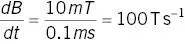
As the gradients are switched, they produce time‐varying magnetic fields . The rate of change of field is given by the derivative of B with respect to time, or dB/dt (measured in T s ‐1). For a trapezoidal gradient waveform ( Figure 1.16)
(1.7) 
where ΔB is the change in B produced by the gradient and Δt is the time over which the change occurs. dB/dt is important when considering acute physiological effects, such as peripheral nerve stimulation (PNS). See Chapter 4 .
Example 1.4 Gradient dB/dt
In the example of Figure 1.16if the peak gradient amplitude is 10 mT and the rise time 0.1 ms, what is the dB/dt?
Radiofrequency field
Figure 1.26shows simulations of the electric and magnetic fields generated around an eight‐rung birdcage transmit coil [5]. The magnetic B 1‐field is highly uniform, whilst the electric field (E) is concentrated around the rungs. In air B 1decreases rapidly beyond the limits of the transmit coil. 2 B 1is produced as a pulse consisting of a “carrier” frequency (at the Larmor frequency) multiplied by a shape or envelope ( Figure 1.27). The simple rectangular pulses of Equation 1.2are seldom used in practice and a more general expression for flip angle is
(1.8) 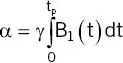
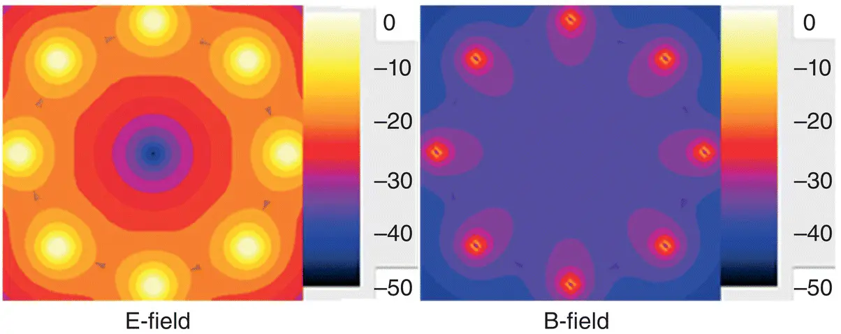
Figure 1.26 Simulated electric (L) and magnetic fields (R) from an eight‐rung birdcage coil. Scale in dB. Source [5], licensee BioMed Central Ltd.
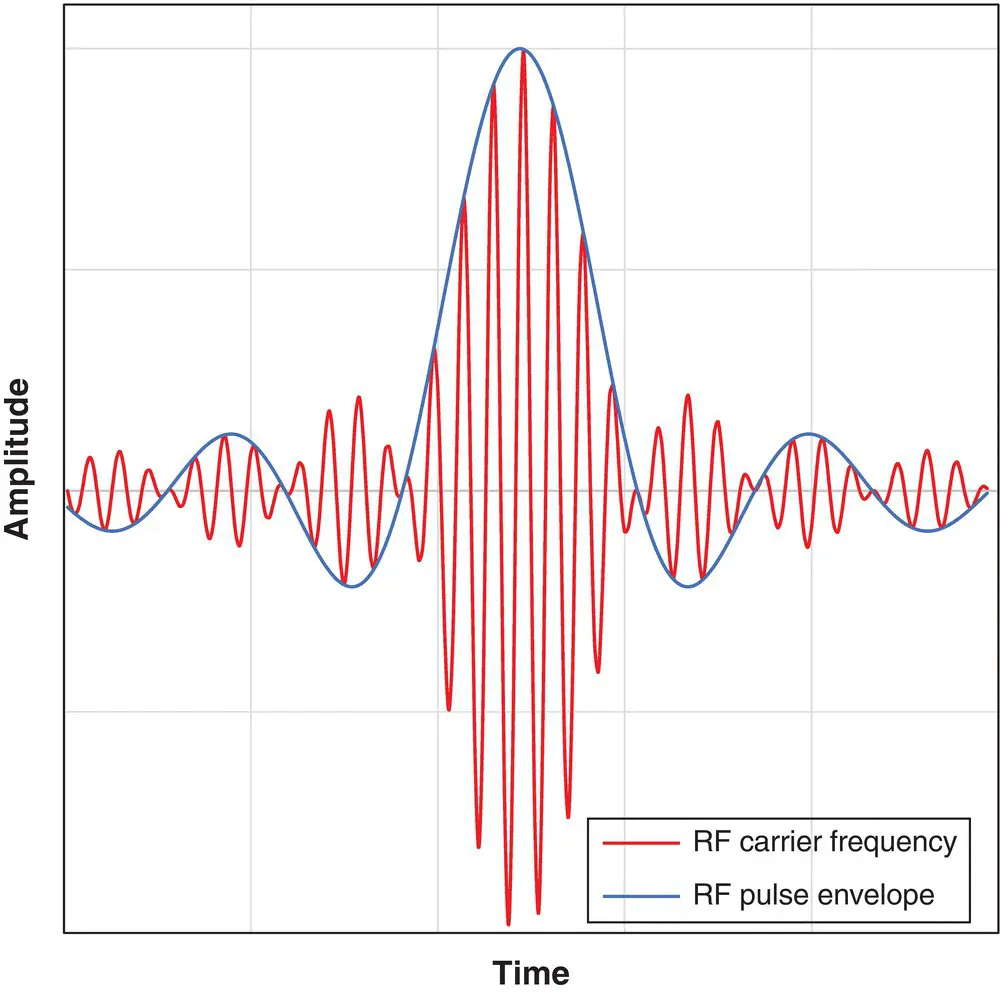
Figure 1.27 RF pulse consisting of the carrier (Larmor) frequency multiplied by a shape function or pulse envelope. The example shown is a truncated sinc (sinx/x) function.
This is equal to the area under the curve of the pulse envelope. Three important points arise:
1 for the same pulse shape and duration, the B1 amplitude is proportional to the flip angle;
2 for the same pulse shape and duration, the B1amplitude required to produce a given flip angle is independent of B0;
Читать дальшеИнтервал:
Закладка:
Похожие книги на «Essentials of MRI Safety»
Представляем Вашему вниманию похожие книги на «Essentials of MRI Safety» списком для выбора. Мы отобрали схожую по названию и смыслу литературу в надежде предоставить читателям больше вариантов отыскать новые, интересные, ещё непрочитанные произведения.


Обсуждение, отзывы о книге «Essentials of MRI Safety» и просто собственные мнения читателей. Оставьте ваши комментарии, напишите, что Вы думаете о произведении, его смысле или главных героях. Укажите что конкретно понравилось, а что нет, и почему Вы так считаете.