Donald W. McRobbie - Essentials of MRI Safety
Здесь есть возможность читать онлайн «Donald W. McRobbie - Essentials of MRI Safety» — ознакомительный отрывок электронной книги совершенно бесплатно, а после прочтения отрывка купить полную версию. В некоторых случаях можно слушать аудио, скачать через торрент в формате fb2 и присутствует краткое содержание. Жанр: unrecognised, на английском языке. Описание произведения, (предисловие) а так же отзывы посетителей доступны на портале библиотеки ЛибКат.
- Название:Essentials of MRI Safety
- Автор:
- Жанр:
- Год:неизвестен
- ISBN:нет данных
- Рейтинг книги:4 / 5. Голосов: 1
-
Избранное:Добавить в избранное
- Отзывы:
-
Ваша оценка:
Essentials of MRI Safety: краткое содержание, описание и аннотация
Предлагаем к чтению аннотацию, описание, краткое содержание или предисловие (зависит от того, что написал сам автор книги «Essentials of MRI Safety»). Если вы не нашли необходимую информацию о книге — напишите в комментариях, мы постараемся отыскать её.
Reflects the most current research, guidelines, and MRI safety information Explains procedures for scanning pregnant women, managing MRI noise exposure, and handling emergency situations Prepares candidates for the American Board of MR Safety exam and other professional certifications Aligns with MRI safety roles such as MR Medical Director (MRMD), MR Safety Officer (MRSO) and MR Safety Expert (MRSE) Contains numerous illustrations, figures, self-assessment tests, key references, and extensive appendices
is an indispensable text for all radiographers and radiologists, as well as physicists, engineers, and researchers with an interest in MRI.
Essentials of MRI Safety — читать онлайн ознакомительный отрывок
Ниже представлен текст книги, разбитый по страницам. Система сохранения места последней прочитанной страницы, позволяет с удобством читать онлайн бесплатно книгу «Essentials of MRI Safety», без необходимости каждый раз заново искать на чём Вы остановились. Поставьте закладку, и сможете в любой момент перейти на страницу, на которой закончили чтение.
Интервал:
Закладка:
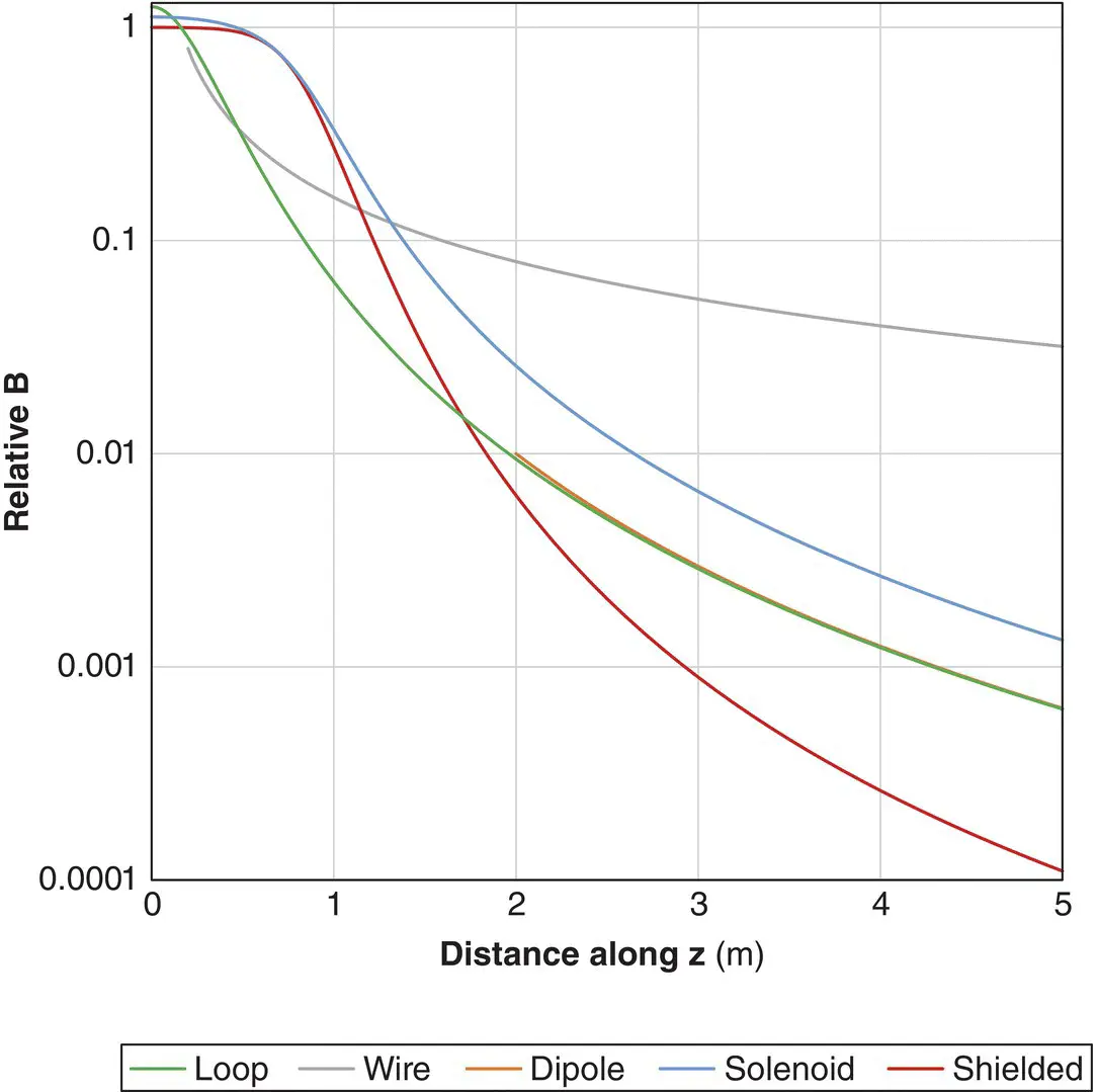
Figure 2.6 Relative magnitude of B zalong the z‐axis for a long straight wire, simple loop, magnetic dipole, solenoid, and simulated self‐shielded magnet with radii of 0.4 m. The iso‐centre is at z = 0.
B field from a solenoidal coil
The field generated at the centre of a solenoid of length d with windings of density N turns per metre ‐ this now looks more like a MR superconducting magnet‐ is
(2.1) 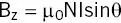
θ is the angle measured from the vertical at iso‐centre to the end of the solenoid ( Figure 2.7). For very long solenoids θ tends to 90° (π/2) and the field is
(2.2) 
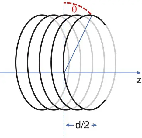
Figure 2.7 Solenoid coil showing the angle θ. For a very long solenoid θ →90°.
This is where the definition of magnetic field strength or intensity H in A m −1(from Chapter 1) comes in, as
(2.3) 
B field from a shielded MRI magnet
The design of a MR magnet (at least for MR safety purposes) can be approximately simulated by two concentric solenoids: the inner one representing the main coil; the outer shield coil has current flowing in the opposite direction. This enables the fringe field to be significantly reduced in extent ( Figure 2.8). It also results in a stronger spatial gradient of B 0, dB/dz, close to the bore entrance, but weaker at greater distance. This poses a significantly increased hazard, as the projectile force on a ferromagnetic object may suddenly increase as you approach the bore entrance – and you only notice when it’s too late. Both B and dB/dz drop off with distance more rapidly than for a dipole (FIGURE 2.6).
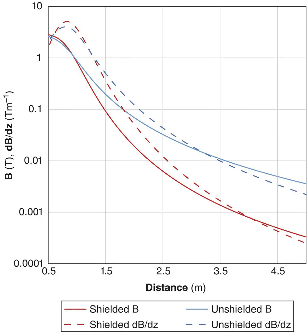
Figure 2.8 B and dB/dt along the axis of a simulated shielded and unshielded 3 T MR magnet. Distances are from the iso‐centre, with the bore entrance at 0.8m. Simulated data for illustration only.
Spatial dependence of magnetic fields
Only the simplest coil geometries can be solved exactly with algebra. A generalized method of computing is given by the Biot‐Savart Law (see Appendix 1). Magnet and gradient coil designers use this to numerically compute the spatial responses of B 0, G x,y,zand B 1fields. It is also used in computer modeling of induced fields in tissue.
MAGNETIC MATERIALS
The previous section showed how a B‐field can be generated in free space or air. Now we consider how materials or physical media respond to an external magnetic field. At the atomic level the electrons in their shells orbiting the nucleus have intrinsic magnetic moments. In most atoms the magnetic moments from the electrons’ spin and orbital motion cancel. This is diamagnetism , the default “non‐magnetic” state. If the cancellation is incomplete then the material is paramagnetic . In ferromagnetic 1 materials, such as iron or steel, the electron spins become aligned in large groups or domains and their effect is significantly greater. Figure 2.9shows the magnetic susceptibility spectrum covering a range of materials [1]. This is an enormous range extending over ten orders of magnitude (10 10); each step in the chart represents a factor of ten.
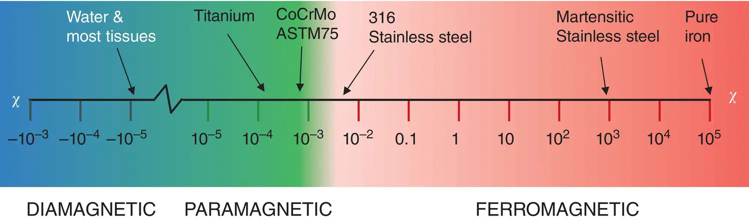
Figure 2.9 Magnetic susceptibility spectrum.
When an object is placed in an external magnetic field, it becomes magnetized. Each of the types of material: dia‐, para‐, and ferromagnetic behave differently in the field, but because of Maxwell’s equations, the underlying physics is similar. In an external field, the magnetization of the material M(a vector) is
(2.4) 
His the magnetic field strength (A m −1) and χ is the magnetic susceptibility which is dimensionless 2 . Table 2.1shows some values of χ .In isotropic media χ is independent of orientation or position and is a simple scalar number. If the material is linear and isotropic we can say
(2.5) 
Table 2.1 Magnetic susceptibility of common materials.
| Type of material | Behavior | Material | χ 1 |
| Diamagnetic | M opposes H and external B 0. Repulsive force. | Water and soft tissueCortical boneDe‐oxygenated red blood cellsCopperSuperconductors | –9.05×10 −6–8.86×10 −6–6.52 ×10 −6–9.63×10 −6–1 |
| Paramagnetic | M parallel to H and external B 0. Attractive force. | AirMagnesiumAluminiumTitaniumCoCrMo alloy | 0.36 ×10 −611.7×10 −620.7×10 −6182×10 −6920×10 −6 |
| Ferromagnetic | M parallel to H and external B 0. Strong attractive force. Can become permanently magnetized. Displays hysteresis. | Martensitic stainless steelSilicon steelMumetalPure iron | ~ 10 310 3–10 410 4–10 5~10 5 |
1Values from [1,2]
The total field within the material is the sum of the external field plus the field resulting from the magnetization of the material.
The relative permeability μ ris also used to characterize magnetic materials
(2.6) 
so
(2.7) 
for linear isotropic materials.
Ferromagnetism
Whilst we will consider (in Chapter 3) the possible consequences of biological effects based upon the dia‐ and para‐ magnetic properties of biological structures, ferromagnetic is the most important class of materials for safety within the MR environment due to the strong magnetic forces. Before we consider these, we need to understand more about ferromagnetism. Figure 2.10shows how the magnetic domains of a ferromagnetic material may align. In the absence of a magnetic field the domains are randomly orientated with no overall magnetization. When an external B‐field (or H) is applied, the domains align and the material becomes highly magnetized. Some materials will retain their magnetism once the external field is removed – these are known as hard ferromagnetic materials, becoming permanent magnets when magnetized. Soft magnetic materials do not retain their domains’ alignment once the external field is removed, or do so to a minor extent which we will neglect.
Читать дальшеИнтервал:
Закладка:
Похожие книги на «Essentials of MRI Safety»
Представляем Вашему вниманию похожие книги на «Essentials of MRI Safety» списком для выбора. Мы отобрали схожую по названию и смыслу литературу в надежде предоставить читателям больше вариантов отыскать новые, интересные, ещё непрочитанные произведения.


Обсуждение, отзывы о книге «Essentials of MRI Safety» и просто собственные мнения читателей. Оставьте ваши комментарии, напишите, что Вы думаете о произведении, его смысле или главных героях. Укажите что конкретно понравилось, а что нет, и почему Вы так считаете.