Ronald J. Anderson - The Practice of Engineering Dynamics

where the directions of the two components are defined. The rate of change of magnitude term is aligned with the position vector and is thus termed radial and the rate of change of direction component is perpendicular to the position vector and is therefore tangential .

Differentiating the velocity expression of Equation 1.45yields,

(1.46)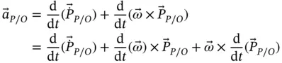

and, applying Equation 1.6to Equation 1.46, we can write,

(1.47)

After collecting terms and substituting (the angular acceleration vector) for , we get the well‐known result,

(1.48)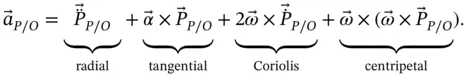

Each of the terms in Equation 1.48has a name and a physical meaning, as follows.

1 is the radial acceleration. This is nothing more than the second derivative of the distance between and and it is aligned with .

2 is the tangential acceleration. It is called the tangential acceleration because it is aligned with the direction in which the point would move if it were a fixed distance from and were rotating about (i.e. in a direction perpendicular to a line passing through and ). Notice that is the total derivative of the angular velocity including its rate of change of magnitude and its rate of change of direction. As a result, may not be aligned with .

3 is the Coriolis acceleration 5 . The vectorial approach to finding the Coriolis acceleration is in many ways preferable to the scalar approach put forward in many books on dynamics. The magnitude of the radial velocity is often referred to in reference books as and the Coriolis acceleration is seen written as where the reader is left to determine its direction from a complicated set of rules. Consideration of Equations 1.45, 1.46, 1.47shows that there are two very different types of terms that combine to form the Coriolis acceleration with its remarkable 2. The two terms are equal in magnitude and direction (i.e. each is ). One of these arises from part of the rate of change of magnitude of the tangential velocity of . The second arises from the rate of change of direction of the radial velocity of .

4 is the centripetal acceleration. In 2D circular motion. this is commonly written as and points toward the center of the circle. For the general points and used here, the centripetal acceleration points from to .

It is possible to visualize the acceleration components using a simple graphical construction. As an example, we can use the slider in a slot system shown in Figure 1.4for which we have already derived both the velocity ( Equation 1.19) and the acceleration ( Equation 1.20) in body fixed coordinates.

Remember that rates of change of magnitude are aligned with the vector that is changing and rates of change of direction are perpendicular to the original vector and are pointed in the direction that the tip of the vector would move if it had the prescribed angular velocity and were simply rotating about its tail.

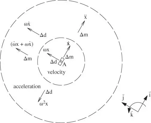
Figure 1.7The velocity and acceleration components of the slider.

Figure 1.7shows the two components of the velocity of the slider in the inner circle. A component is labeled with a to indicate that it results from a rate of change of magnitude or a to show that it results from a rate of change of direction. The two terms here are the radial velocity aligned with the original position vector (a rate of change of magnitude term) and the tangential velocity (a rate of change of direction term) perpendicular to the position vector, pointing in the direction that the angular velocity would cause point to move if it were simply rotating about , and with magnitude equal to the vector length multiplied by the angular speed. These are the same two terms that appear in Equation 1.19.

Between the inner and outer circles on Figure 1.7are the components of the acceleration. To get these terms, we treat the velocity components as separate vectors that can change in magnitude and direction and apply to each of them the same procedure we used on the position vector in the preceding paragraph.

Consider first the radial velocity ( ). Its rate of change of magnitude will be aligned with it and will be equal to the rate of change of its length (i.e. the derivative of with respect to time or ). As we watch it rotate about its tail with angular speed , the tip of this vector will move at the rate in the direction shown on the figure. This rate of change of direction of the radial velocity is one half of the Coriolis acceleration.

Next consider the tangential velocity ( ). Its rate of change of magnitude is aligned with it and consists of the time derivative of which has two terms by the chain rule of differentiation (i.e. and ). Notice that the second of these terms is the other half of the Coriolis acceleration. The rate of change of direction of the tangential velocity is found by rotating it about its tail with angular speed and finding that it has magnitude or and points from to . The rate of change of direction of the tangential velocity is, in fact, the centripetal acceleration.