Samprit Chatterjee - Handbook of Regression Analysis With Applications in R

A final way of comparing models is from a directly predictive point of view. Since a rough prediction interval is , a useful model from a predictive point of view is one with small , suggesting choosing a model that has small while still being as simple as possible. That is,

1 Increase the number of predictors until levels off. For these data ( in the output refers to ), this implies choosing or .

Taken together, all of these rules imply that the appropriate set of models to consider are those with two, three, or four predictors. Typically, the strongest model of each size (which will have highest , highest , lowest , lowest , and lowest , so there is no controversy as to which one is strongest) is examined. The output on pages 31–32 provides summaries for the top three models of each size, in case there are reasons to examine a second‐ or third‐best model (if, for example, a predictor in the best model is difficult or expensive to measure), but here we focus on the best model of each size. First, here is output for the best four‐predictor model.

Coefficients: Estimate Std.Error t value Pr(>|t|) VIF (Intercept) -6.852e+06 3.701e+06 -1.852 0.0678 . Bedrooms -1.207e+04 9.212e+03 -1.310 0.1940 1.252 Bathrooms 5.303e+04 1.275e+04 4.160 7.94e-05 1.374 *** Living.area 6.828e+01 1.460e+01 4.676 1.17e-05 1.417 *** Year.built 3.608e+03 1.898e+03 1.901 0.0609 1.187 . --- Signif. codes: 0 ‘***’ 0.001 ‘**’ 0.01 ‘*’ 0.05 ‘.’ 0.1 ‘ ’ 1 Residual standard error: 46890 on 80 degrees of freedom Multiple R-squared: 0.5044, Adjusted R-squared: 0.4796 F-statistic: 20.35 on 4 and 80 DF, p-value: 1.356e-11

The ‐statistic for number of bedrooms suggests very little evidence that it adds anything useful given the other predictors in the model, so we consider now the best three‐predictor model. This happens to be the best four‐predictor model with the one statistically insignificant predictor omitted, but this does not have to be the case.

Coefficients: Estimate Std.Error t value Pr(>|t|) VIF (Intercept) -7.653e+06 3.666e+06 -2.087 0.039988 * Bathrooms 5.223e+04 1.279e+04 4.084 0.000103 1.371 *** Living.area 6.097e+01 1.355e+01 4.498 2.26e-05 1.210 *** Year.built 4.001e+03 1.883e+03 2.125 0.036632 1.158 * --- Signif. codes: 0 ‘***’ 0.001 ‘**’ 0.01 ‘*’ 0.05 ‘.’ 0.1 ‘ ’ 1 Residual standard error: 47090 on 81 degrees of freedom Multiple R-squared: 0.4937, Adjusted R-squared: 0.475 F-statistic: 26.33 on 3 and 81 DF, p-value: 5.489e-12

Each of the predictors is statistically significant at a level, and this model recovers virtually all of the available fit ( , while that using all six predictors is ), so this seems to be a reasonable model choice. The estimated slope coefficients are very similar to those from the model using all predictors (which is not surprising given the low collinearity in the data), so the interpretations of the estimated coefficients on page 17 still hold to a large extent. A plot of the residuals versus the fitted values and a normal plot of the residuals ( Figure 2.2) look fine, and similar to those for the model using all six predictors in Figure 1.5; plots of the residuals versus each of the predictors in the model are similar to those in Figure 1.6, so they are not repeated here.

Once a “best” model is chosen, it is tempting to use the usual inference tools (such as ‐tests and ‐tests) to try to explain the process being studied. Unfortunately, doing this while ignoring the model selection process can lead to problems. Since the model was chosen to be best (in some sense) it will tend to appear stronger than would be expected just by random chance. Conducting inference based on the chosen model as if it was the only one examined ignores an additional source of variability, that of actually choosing the model (model selection based on a different sample from the same population could very well lead to a different chosen “best” model). This is termed model selection uncertainty. As a result of ignoring model selection uncertainty, confidence intervals can have lower coverage than the nominal value, hypothesis tests can reject the null too often, and prediction intervals can be too narrow for their nominal coverage.

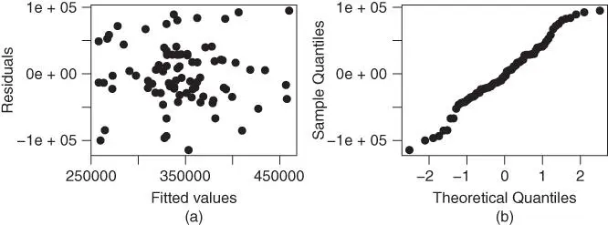
FIGURE 2.2: Residual plots for the home price data using the best three‐predictor model. (a) Plot of residuals versus fitted values. (b) Normal plot of the residuals.

Identifying and correcting for this uncertainty is a difficult problem, and an active area of research, and will be discussed further in Chapter 14. There are, however, a few things practitioners can do. First, it is not appropriate to emphasize too strongly the single “best” model; any model that has similar criteria values (such as or ) to those of the best model should be recognized as being one that could easily have been chosen as best based on a different sample from the same population, and any implications of such a model should be viewed as being as valid as those from the best model. Further, one should expect that ‐values for the predictors included in a chosen model are potentially smaller than they should be, so taking a conservative attitude regarding statistical significance is appropriate. Thus, for the chosen three‐predictor model summarized on page 35, number of bathrooms and living area are likely to correspond to real effects, but the reality of the year built effect is more questionable.