Samprit Chatterjee - Handbook of Regression Analysis With Applications in R

1 Choose the model that minimizes . In case of tied values, the simplest model (smallest ) would be chosen. In these data, this rule implies choosing .

An additional operational rule for the use of has been suggested. When a particular model contains all of the necessary predictors, the residual mean square for the model should be roughly equal to . Since the model that includes all of the predictors should also include all of the necessary ones, should also be roughly equal to . This implies that if a model includes all of the necessary predictors, then

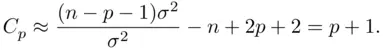
This suggests the following model selection rule:

1 Choose the simplest model such that or smaller. In these data, this rule implies choosing .

A weakness of the criterion is that its value depends on the largest set of candidate predictors (through ), which means that adding predictors that provide no predictive power to the set of candidate models can change the choice of best model. A general approach that avoids this is through the use of statistical information. A detailed discussion of the determination of information measures is beyond the scope of this book, but Burnham and Anderson (2002) provides extensive discussion of the topic. The Akaike Information Criterion , introduced by Akaike (1973),

(2.2)

where the function refers to natural logs, is such a measure, and it estimates the information lost in approximating the true model by a candidate model. It is clear from (2.2)that minimizing achieves the goal of balancing strength of fit with simplicity, and because of the term in the criterion this will result in the choice of similar models as when minimizing . It is well known that has a tendency to lead to overfitting, particularly in small samples. That is, the penalty term in designed to guard against too complicated a model is not strong enough. A modified version of that helps address this problem is the corrected ,

(2.3)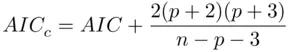

(Hurvich and Tsai, 1989). Equation (2.3)shows that (especially for small samples) models with fewer parameters will be more strongly preferred when minimizing than when minimizing , providing stronger protection against overfitting. In large samples, the two criteria are virtually identical, but in small samples, or when considering models with a large number of parameters, is the better choice. This suggests the following model selection rule:

1 Choose the model that minimizes . In case of tied values, the simplest model (smallest ) would be chosen. In these data, this rule implies choosing , although the value for is virtually identical to that of . Note that the overall level of the values is not meaningful, and should not be compared to values or values for other data sets; it is only the value for a model for a given data set relative to the values of others for that data set that matter.

, , and have the desirable property that they are efficient model selection criteria. This means that in the (realistic) situation where the set of candidate models does not include the “true” model (that is, a good model is just viewed as a useful approximation to reality), as the sample gets larger the error obtained in making predictions using the model chosen using these criteria becomes indistinguishable from the error obtained using the best possible model among all candidate models. That is, in this large‐sample predictive sense, it is as if the best approximation was known to the data analyst. Another well‐known criterion, the Bayesian Information Criterion [which substitutes for in (2.2)], does not have this property, but is instead a consistent criterion. Such a criterion has the property that if the “true” model is in fact among the candidate models the criterion will select that model with probability approaching as the sample size increases. Thus, is a more natural criterion to use if the goal is to identify the “true” predictors with nonzero slopes (which of course presumes that there are such things as “true” predictors in a “true” model). will generally choose simpler models than because of its stronger penalty ( for ), and a version that adjusts as in (2.3)leads to even simpler models. This supports the notion that from a predictive point of view including a few unnecessary predictors (overfitting) is far less damaging than is omitting necessary predictors (underfitting).