Samprit Chatterjee - Handbook of Regression Analysis With Applications in R

Note that model comparisons are only sensible when based on the same data set. Most statistical packages drop any observations that have missing data in any of the variables in the model. If a data set has missing values scattered over different predictors, the set of observations with complete data will change depending on which variables are in the model being examined, and model comparison measures will not be comparable. One way around this is to only use observations with complete data for all variables under consideration, but this can result in discarding a good deal of available information for any particular model.

Tools like best subsets by their very nature are likely to be more effective when there are a relatively small number of useful predictors that have relatively strong effects, as opposed to a relatively large number of predictors that have relatively weak effects. The strict present/absent choice for a predictor is consistent with true relationships with either zero or distinctly nonzero slopes, as opposed to many slopes that are each nonzero but also not far from zero.

Consider again the home price data examined in Section 1.4. We repeat the regression output from the model based on all of the predictors below:

Coefficients: Estimate Std.Error t value Pr(>|t|) VIF (Intercept) -7.149e+06 3.820e+06 -1.871 0.065043 . Bedrooms -1.229e+04 9.347e+03 -1.315 0.192361 1.262 Bathrooms 5.170e+04 1.309e+04 3.948 0.000171 1.420 *** Living.area 6.590e+01 1.598e+01 4.124 9.22e-05 1.661 *** Lot.size -8.971e-01 4.194e+00 -0.214 0.831197 1.074 Year.built 3.761e+03 1.963e+03 1.916 0.058981 1.242 . Property.tax 1.476e+00 2.832e+00 0.521 0.603734 1.300 --- Signif. codes: 0 ‘***’ 0.001 ‘**’ 0.01 ‘*’ 0.05 ‘.’ 0.1 ‘ ’ 1 Residual standard error: 47380 on 78 degrees of freedom Multiple R-squared: 0.5065, Adjusted R-squared: 0.4685 F-statistic: 13.34 on 6 and 78 DF, p-value: 2.416e-10

This is identical to the output given earlier, except that variance inflation factor ( ) values are given for each predictor. It is apparent that there is virtually no collinearity among these predictors (recall that is the minimum possible value of the ), which should make model selection more straightforward. The following output summarizes a best subsets fitting:

P L r i Y o B v e p B a i L a e e t n o r r d h g t . t r r . . b y o o a s u . o o r i i t Mallows m m e z l a Vars R-Sq R-Sq(adj) Cp AICc S s s a e t x 1 35.3 34.6 21.2 1849.9 52576 X 1 29.4 28.6 30.6 1857.3 54932 X 1 10.6 9.5 60.3 1877.4 61828 X 2 46.6 45.2 5.5 1835.7 48091 X X 2 38.9 37.5 17.5 1847.0 51397 X X 2 37.8 36.3 19.3 1848.6 51870 X X 3 49.4 47.5 3.0 1833.1 47092 X X X 3 48.2 46.3 4.9 1835.0 47635 X X X 3 46.6 44.7 7.3 1837.5 48346 X X X 4 50.4 48.0 3.3 1833.3 46885 X X X X 4 49.5 47.0 4.7 1834.8 47304 X X X X 4 49.4 46.9 5.0 1835.1 47380 X X X X 5 50.6 47.5 5.0 1835.0 47094 X X X X X 5 50.5 47.3 5.3 1835.2 47162 X X X X X 5 49.6 46.4 6.7 1836.8 47599 X X X X X 6 50.6 46.9 7.0 1836.9 47381 X X X X X X

Output of this type provides the tools to choose among candidate models. The output provides summary statistics for the three models with strongest fit for each number of predictors. So, for example, the best one‐predictor model is based on Bathrooms, while the second best is based on Living.area; the best two‐predictor model is based on Bathroomsand Living.area; and so on. The principle of parsimony noted earlier implies moving down the table as long as the gain in fit is big enough, but no further, thereby encouraging simplicity. A reasonable model selection strategy would not be based on only one possible measure, but looking at all of the measures together, using various guidelines to ultimately focus in on a few models (or only one) that best trade off strength of fit with simplicity, for example as follows:

1 Increase the number of predictors until the value levels off. Clearly, the highest for a given cannot be smaller than that for a smaller value of . If levels off, that implies that additional variables are not providing much additional fit. In this case, the largest values go from roughly to from to , which is clearly a large gain in fit, but beyond that more complex models do not provide much additional fit (particularly past ). Thus, this guideline suggests choosing either or .

2 Choose the model that maximizes the adjusted . Recall from equation (1.7)that the adjusted equalsIt is apparent that explicitly trades off strength of fit () versus simplicity [the multiplier ], and can decrease if predictors that do not add any predictive power are added to a model. Thus, it is reasonable to not complicate a model beyond the point where its adjusted increases. For these data, is maximized at .

The fourth column in the output refers to a criterion called Mallows' (Mallows, 1973). This criterion equals

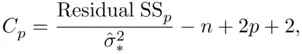
where is the residual sum of squares for the model being examined, is the number of predictors in that model, and is the residual mean square based on using all of the candidate predicting variables. is designed to estimate the expected squared prediction error of a model. Like , explicitly trades off strength of fit versus simplicity, with two differences: it is now small values that are desirable, and the penalty for complexity is stronger, in that the penalty term now multiplies the number of predictors in the model by , rather than by (which means that using will tend to lead to more complex models than using will). This suggests another model selection rule: