Samprit Chatterjee - Handbook of Regression Analysis With Applications in R

There is a straightforward way to get a sense of the predictive power of a chosen model if enough data are available. This can be evaluated by holding out some data from the analysis (a holdoutor validationsample), applying the selected model from the original data to the holdout sample (based on the previously estimated parameters, not estimates based on the new data), and then examining the predictive performance of the model. If, for example, the standard deviation of the errors from this prediction is not very different from the standard error of the estimate in the original regression, chances are making inferences based on the chosen model will not be misleading. Similarly, if a (say) prediction interval does not include roughly of the new observations, that indicates poorer‐than‐expected predictive performance on new data.

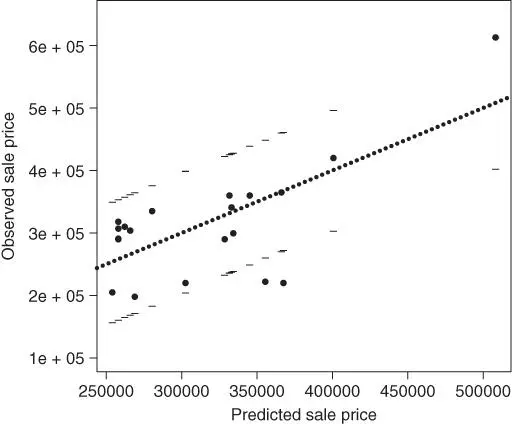
FIGURE 2.3: Plot of observed versus predicted house sale price values of validation sample, with pointwise prediction interval limits superimposed. The dotted line corresponds to equality of observed values and predictions.

Figure 2.3illustrates a validation of the three‐predictor housing price model on a holdout sample of houses. The figure is a plot of the observed versus predicted prices, with pointwise prediction interval limits superimposed. The intervals contain of the prices ( of ), and the average predictive error on the new houses is only (compared to an average observed price of more than ), not suggesting the presence of any forecasting bias in the model. Two of the houses, however, have sale prices well below what would have been expected (more than lower than expected), and this is reflected in a much higher standard deviation ( ) of the predictive errors than from the fitted regression. If the two outlying houses are omitted, the standard deviation of the predictive errors is much smaller ( ), suggesting that while the fitted model's predictive performance for most houses is in line with its performance on the original sample, there are indications that it might not predict well for the occasional unusual house.

If validating the model on new data this way is not possible, a simple adjustment that is helpful is to estimate the variance of the errors as

(2.4)

where is based on the chosen “best” model, and is the number of predictors in the most complex model examined, in the sense of most predictors (Ye, 1998). Clearly, if very complex models are included among the set of candidate models, can be much larger than the standard error of the estimate from the chosen model, with correspondingly wider prediction intervals. This reinforces the benefit of limiting the set of candidate models (and the complexity of the models in that set) from the start. In this case , so the effect is not that pronounced.

The adjustment of the denominator in (2.4)to account for model selection uncertainty is just a part of the more general problem that standard degrees of freedom calculations are no longer valid when multiple models are being compared to each other as in the comparison of all models with a given number of predictors in best subsets. This affects other uses of those degrees of freedom, including the calculation of information measures like , , , and , and thus any decisions regarding model choice. This problem becomes progressively more serious as the number of potential predictors increases and is the subject of active research. This will be discussed further in Chapter 14.

It is not unusual for the observations in a sample to fall into two distinct subgroups; for example, people are either male or female. It might be that group membership has no relationship with the target variable (given other predictors); such a pooled modelignores the grouping and pools the two groups together.

On the other hand, it is clearly possible that group membership is predictive for the target variable (for example, expected salaries differing for men and women given other control variables could indicate gender discrimination). Such effects can be explored easily using an indicator variable, which takes on the value for one group and for the other (such variables are sometimes called dummy variablesor variables). The model takes the form