Samprit Chatterjee - Handbook of Regression Analysis With Applications in R

for counties that did not use electronic voting in 2004, and

for counties that did use electronic voting. This is represented in Figure 2.5. This relationship implies that in counties that did not use electronic voting the more Republican a county was in 2000, the larger the gain for Bush in 2004, while in counties with electronic voting, the opposite pattern held true.

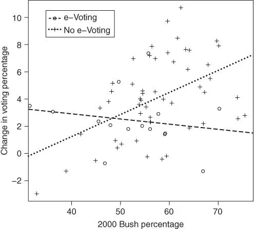
FIGURE 2.5: Regression lines for election data separated by whether the county used electronic voting in 2004.

As can be seen from the VIFs, the predictor and the product variable are collinear. This isn't very surprising, since one is a function of the other, and such collinearity is more likely to occur if one of the subgroups is much larger than the other, or if group membership is related to the level or variability of the predictor variable. Given that using the product variable is just a computational construction that allows the fitting of two separate regression lines, this is not a problem in this context.

This model is probably underspecified, as it does not include control variables that would be expected to be related to voting percentage. Figure 2.6gives scatter plots of the percentage change in Bush votes versus (a) the total county voter turnouts in 2000 and (b) 2004, (c) median income, and (d) percentage of the voters being Hispanic. None of the marginal relationships are very strong, but in the multiple regression summarized below, median income does seem to add important predictive power without changing the previous relationships between change in Bush voting percentage and 2000 Bush percentage very much.

Coefficients: Estimate Std.Error t val P(>|t|) VIF (Intercept) 1.166e+00 2.55e+00 0.46 0.650 Bush.pct.2000 1.639e-01 3.69e-02 4.45 3.9e-5 1.55 *** e.Voting 1.426e+01 4.84e+00 2.95 0.005 54.08 ** Bush.2000 X e.Voting -2.545e-01 8.47e-02 -3.01 0.004 47.91 ** Vote.turn.2000 -5.957e-06 3.10e-05 -0.19 0.848 210.66 Vote.turn.2004 1.413e-06 2.49e-05 0.06 0.955 205.81 Median.income -1.745e-04 5.61e-05 -3.11 0.003 1.66 ** Hispan.pop.pct -4.127e-02 3.18e-02 -1.30 0.200 1.32 --- Signif. codes: 0 ‘***’ 0.001 ‘**’ 0.01 ‘*’ 0.05 ‘.’ 0.1 ‘ ’ 1 Residual standard error: 2.244 on 59 degrees of freedom Multiple R-squared: 0.4624, Adjusted R-squared: 0.3986 F-statistic: 7.25 on 7 and 59 DF, p-value: 2.936e-06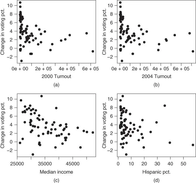

FIGURE 2.6: Plots for the 2004 election data. (a) Plot of percentage change in Bush vote versus 2000 voter turnout. (b) Plot of percentage change in Bush vote versus 2004 voter turnout. (c) Plot of percentage change in Bush vote versus median income. (d) Plot of percentage change in Bush vote versus percentage Hispanic voters.

We could consider simplifying the model here, but often researchers prefer to not remove control variables, even if they do not add to the fit, so that they can be sure that the potential effect is accounted for. This is generally not unreasonable if collinearity is not a problem, but control variables that do not provide additional significant predictive power, but are collinear with the variables that are of direct interest, might be worth removing so they don't obscure the relationships involving the more important variables. In these data the two voter turnout variables are (not surprisingly) highly collinear, but a potential simplification to consider (particularly given that the target variable is the change in Bush voting percentage from 2000 to 2004) is to consider the change in voter turnout as a predictor (the fact that the estimated slope coefficients for 2000 and 2004 voter turnout are of opposite signs and not very different also supports this idea). The model using change in voter turnout is a subset of the model using 2000 and 2004 voter turnout separately (corresponding to restriction ), so the two models can be compared using a partial ‐test. As can be seen below, the fit of the simpler model is similar to that of the more complicated one, collinearity is no longer a problem, and it turns out that the partial ‐test ( , ) supports that the simpler model fits well enough compared to the more complicated model to be preferred (although voter turnout is still apparently not important).

Coefficients: Estimate Std.Error t val P(>|t|) VIF (Intercept) 1.157e+00 2.54e+00 0.46 0.651 Bush.pct.2000 1.633e-01 3.67e-02 4.46 3.7e-05 1.55 *** e.Voting 1.272e+01 4.20e+00 3.03 0.004 41.25 ** Bush.2000 X e.Voting -2.297e-01 7.53e-02 -3.05 0.003 38.25 ** Change.turnout -1.223e-05 1.36e-05 -0.90 0.370 2.44 Median.income -1.718e-04 5.57e-05 -3.08 0.003 1.65 ** Hispan.pop.pct -4.892e-02 2.94e-02 -1.66 0.102 1.14 --- Signif. codes: 0 ‘***’ 0.001 ‘**’ 0.01 ‘*’ 0.05 ‘.’ 0.1 ‘ ’ 1 Residual standard error: 2.233 on 60 degrees of freedom Multiple R-squared: 0.4585, Adjusted R-squared: 0.4044 F-statistic: 8.468 on 6 and 60 DF, p-value: 1.145e-06

Residual plots given in Figure 2.7do not indicate any obvious problems, although the potential nonconstant variance related to whether a county used electronic voting or not noted in Figure 2.4is still indicated. We will not address that issue here, but correction of nonconstant variance related to subgroups in the data will be discussed in Section 6.3.3.

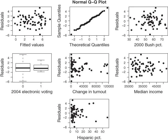
FIGURE 2.7: Residual plots for the 2004 election data.

In this chapter, we have discussed various issues related to model building and model selection. Such methods are important because both underfitting (not including variables that are needed) and overfitting (including variables that are not needed) lead to problems in interpreting the results of regression analyses and making predictions using fitted regression models. Hypothesis tests provide one tool for model building through formal comparisons of models. If one model is a special case of another, defined through a linear restriction, then a partial ‐statistic provides a test of whether the more complex model provides significantly more predictive power than does the simpler one. One important example of a partial ‐test is the standard ‐test for the significance of a slope coefficient. Another important use of partial ‐tests is in the construction of models for data where observations fall into two distinct subgroups that allow for common (pooled) relationships over groups, constant shift relationships that differ only in level but not in slopes, and completely distinct and different relationships across groups.