Muhammad Aslam - Introduction to Statistical Process Control

The science of statistics is based on a number of probability distributions used to measure the likelihood of a particular phenomenon. Two types of random variables are considered in the control chart literature, i.e. continuous random variable and the discrete random variable. A continuous random variable is one which can assume each and every possible value in a given interval, for example, height, weight, temperature, etc. Whereas a discrete variable can assume only some specific integer or whole number value as it deals with the counting of the numbers, for example, yes/no, good/defective, go/no go, etc.

In the domain of the SPC, mostly we collect the random data on continuous scale (Oakland, 2008). The likelihood of this continuous scale data can be best studied through the normal probability distribution. It is a bell‐shaped distribution with the mean at the center and its spread; the width of the curve is reflected by its standard deviation. Due to some nice properties, it is commonly used by the quality control personnel. In SPC the normal probability distribution helps us to determine the probability of falling an observation within the control limits and out of the control limits. If x is the normal random variable, then the probability distribution of x can be defined as

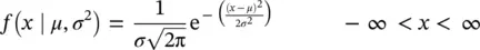
The mean of the normal distribution is μ (− ∞ < μ < ∞), and the variance is σ 2> 0. This distribution is commonly used as x ~ N ( μ , σ 2) to describe that x is normally distributed with mean μ and variance σ 2.

The cumulative normal distribution may be defined as the probability that the random variable x is less than or equal to some arbitrarily value a , which is

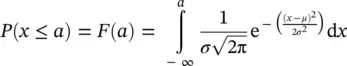
The solution of this integral cannot be computed in closed form. However, by using the transformation of the variable x as

with zero mean and unit variance and known as standard normal distribution. When this transformation takes place, the area of the random variable from the non‐normal distribution is the same as that of the area of the standard normal distribution. The evaluation can be made independent of μ and σ 2; then this probability can be written as

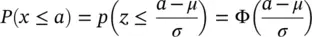
where Φ(·) is the cumulative distribution function of the standard normal distribution with mean 0 and unit variance (Montgomery, 2009). The areas or the probabilities can be computed using the table of areas under standard normal distribution given in Appendix A.

The graph of the normal distribution is called the normal curve. The normal probability distribution has the following important properties ( Figure 1.2):

1 The range of the normal random variable is −∞, +∞.

2 This distribution is bell shaped and symmetric about mean.

3 The mean, median, and mode of the normal distribution are same.

4 The total area/probability under the normal curve is one.

5 All odd order moments about mean are zero.

6 The normal curve extended to both sides of the mean but never touches the x‐axis.

7 The area under the normal curve from

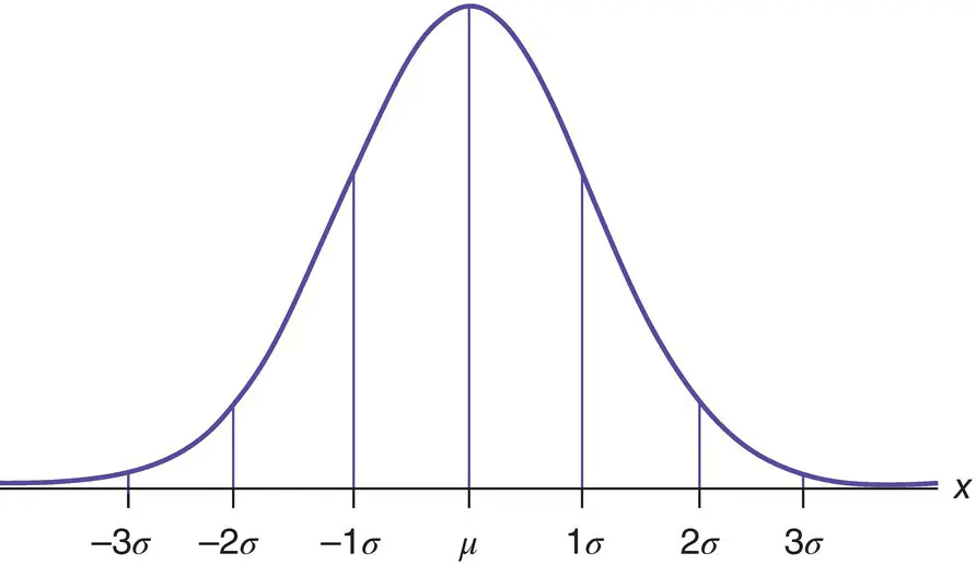
Figure 1.2 Standard normal curve.

Source: https://www.google.com/search?q=Standard+normal+curve&safe=strict&rlz=1C1CHBD_enSA905SA905&sxsrf=ALeKk038CFj1c5F9mxFymaEMSjV1xUEkzA:1592774965148&tbm=isch&source=iu&ictx=1&fir=PAgPMxS8fXpb_M%253A%252CrrsoLwiuhUAKeM%252C_&vet=1&usg=AI4_−kQqYcq7FaH5CrTe620‐F‐8cvWw6Bg&sa=X&ved=2ahUKEwjdr4SQ7ZPqAhVRPJoKHQTVC50Q_h0wAXoECAcQBg&biw=1280&bih=631#imgrc=PAgPMxS8fXpb_M:

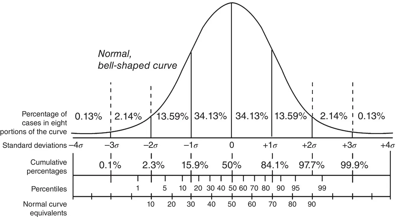
Figure 1.3 Standard normal curve.

Source: https://www.google.com/search?q=Standard+normal+curve&safe=strict&rlz=1C1CHBD_enSA905SA905&sxsrf=ALeKk038CFj1c5F9mxFymaEMSjV1xUEkzA:1592774965148&tbm=isch&source=iu&ictx=1&fir=PAgPMxS8fXpb_M%253A%252CrrsoLwiuhUAKeM%252C_&vet=1&usg=AI4_−kQqYcq7FaH5CrTe620‐F‐8cvWw6Bg&sa=X&ved=2ahUKEwjdr4SQ7ZPqAhVRPJoKHQTVC50Q_h0wAXoECAcQBg&biw=1280&bih=631#imgrc=PAgPMxS8fXpb_M:

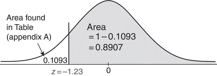
Figure 1.4 Standard normal curve.

Source: https://www.google.com/search?q=Standard+normal+curve&safe=strict&rlz=1C1CHBD_enSA905SA905&sxsrf=ALeKk038CFj1c5F9mxFymaEMSjV1xUEkzA:1592774965148&tbm=isch&source=iu&ictx=1&fir=PAgPMxS8fXpb_M%253A%252CrrsoLwiuhUAKeM%252C_&vet=1&usg=AI4_−kQqYcq7FaH5CrTe620‐F‐8cvWw6Bg&sa=X&ved=2ahUKEwjdr4SQ7ZPqAhVRPJoKHQTVC50Q_h0wAXoECAcQBg&biw=1280&bih=631#imgrc=PAgPMxS8fXpb_M:

Different areas under the normal curve can be calculated as given in Figure 1.3.

To calculate the area Z ≥ − 1.23, we proceed by identifying the area on the normal curve as given in Figure 1.4.

To calculate the area between that −2.00 ≤ Z ≤ 1.50, we proceed by identifying the area on the normal curve as shown in Figure 1.5.

The standard normal distribution has the following important properties:

1 The cumulative area for the Z‐score equal to −3.49 is close to 0.

2 The cumulative area for the Z‐score increases as the value of Z‐score increases.

3 The cumulative area for the Z‐score equal to 0 is 0.50.

4 The cumulative area for the Z‐score equal to 3.49 is close to 1.

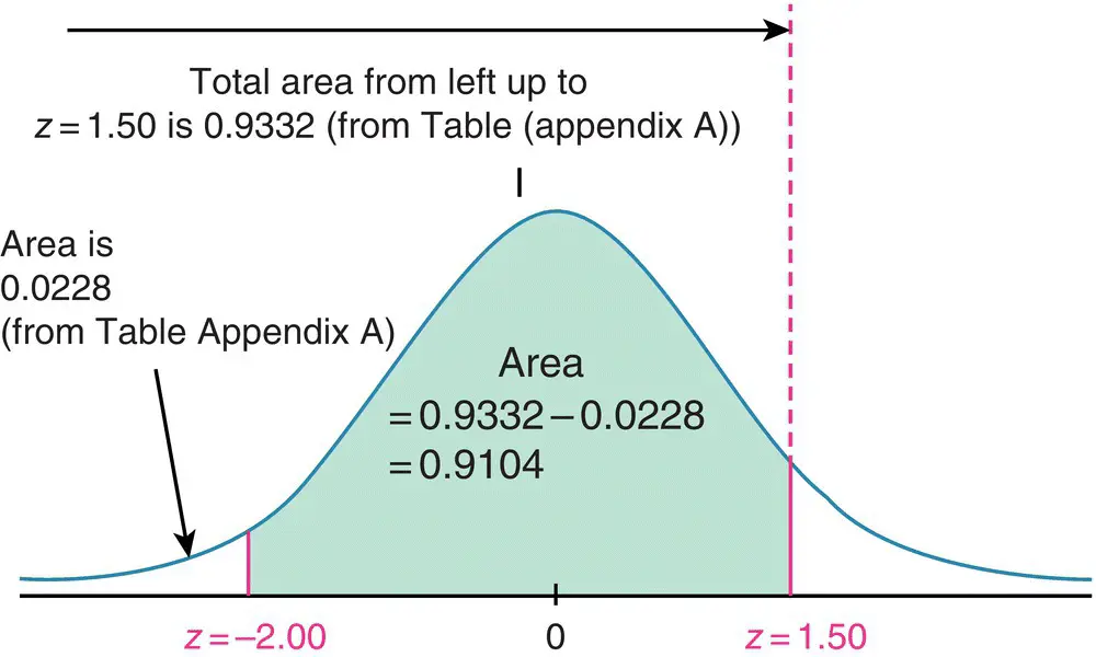
Figure 1.5 Standard normal curve.

Source: https://www.google.com/search?q=Standard+normal+curve&safe=strict&rlz=1C1CHBD_enSA905SA905&sxsrf=ALeKk038CFj1c5F9mxFymaEMSjV1xUEkzA:1592774965148&tbm=isch&source=iu&ictx=1&fir=PAgPMxS8fXpb_M%253A%252CrrsoLwiuhUAKeM%252C_&vet=1&usg=AI4_−kQqYcq7FaH5CrTe620‐F‐8cvWw6Bg&sa=X&ved=2ahUKEwjdr4SQ7ZPqAhVRPJoKHQTVC50Q_h0wAXoECAcQBg&biw=1280&bih=631#imgrc=PAgPMxS8fXpb_M:

Another most commonly used probability distribution is the Student's t ‐distribution, which was discovered by the English statistician William Sealy Gossett (1876–1937), when he published his paper with the pseudonym, “Student.” This distribution is used for the estimation of the population mean when a sample of v assumed to be normally distributed from that population. If x is a random variable, then the heavy tailed symmetrical t ‐distribution is defined as

with mean zero and variance