Sindo Kou - Welding Metallurgy

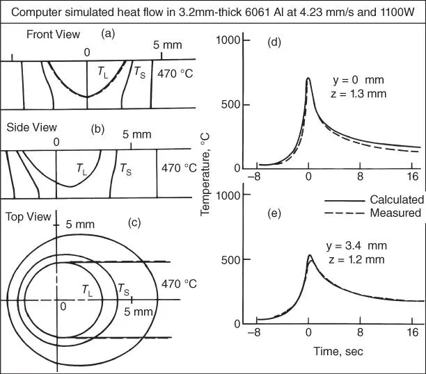
Figure 2.24Computer simulation of GTAW of 3.2‐mm‐thick 6061 Al, 110 A, 10 V, and 4.23 mm/s: (a) fusion boundaries and isotherms; (b) thermal cycles.

Source : Kou and Le [24]. © TMS.

Figure 2.25shows the results of computer simulation of Kou and Le [24] on the effect of the power density distribution of the heat source on the weld shape. Under the same heat input and welding speed, weld penetration decreases with decreasing power density of the heat source. In the computer simulation, the power density distribution at the workpiece surface is approximated by the following Gaussian distribution:

(2.12)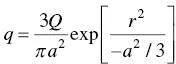

where q is the power density, Q the rate of heat transfer from the heat source to the workpiece, r is the radial distance at the workpiece surface from the centerline of the heat source, and a is the effective radius of the heat source. As shown previously in Figure 2.13, the measured power density distribution is close to a Gaussian distribution.

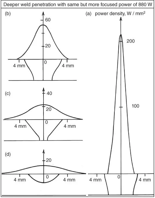
Figure 2.25Effect of power density distribution on weld shape in GTAW of 3.2‐mm 6061 aluminum with 880 W and 4.23 mm/s.

Source : Kou and Le [24]. © TMS.

The thermal cycles experienced by the workpiece during welding can be duplicated in small specimens using a weld thermal simulator called Gleeble. These simulators evolved from an original device developed by Nippes and Savage in 1949 [62]. Figure 2.26shows a specimen being resistance heated by the electric current passing through the specimen and the water‐cooled jaws holding it [63]. A thermocouple spot welded to the middle of the specimen surface is connected to a feedback control system that controls the amount of electric current passing through the specimen such that a specific thermal cycle can be duplicated. A heating rate as high as 10 000 °C/s can be achieved.

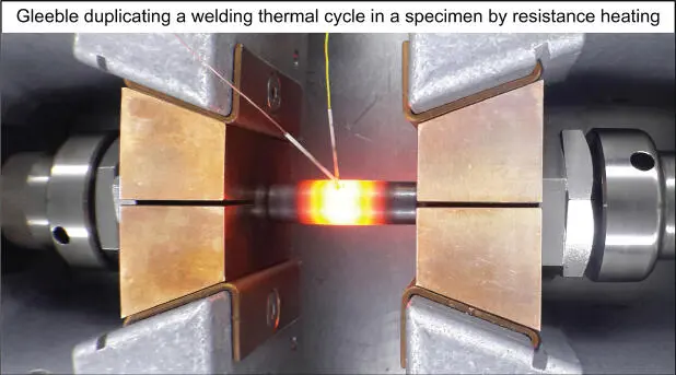
Figure 2.26The thermal cycle at any location in a weld can be duplicated in the specimen with the help of a thermocouple and the thermal simulator.

Source : Courtesy of Dynamic Systems Inc.

There are many applications for weld thermal simulators. For instance, a weld thermal simulator can be used in conjunction with a high‐speed dilatometer to help construct continuous‐cooling transformation diagrams useful for studying phase transformations in welding and heat treating of steels.

By performing high‐speed tensile testing during weld thermal simulation, the elevated‐temperature ductility and strength of metals can be evaluated. This is often called the hot‐ductility test. Nippes and Savage [64, 65], for instance, used this test to investigate the HAZ fissuring in austenitic stainless steels.

Charpy impact test specimens can also be prepared from specimens (1 cm by 1 cm in cross section) subjected to various thermal cycles. This synthetic‐specimen or simulated‐microstructure technique has been employed by numerous investigators to study the HAZ toughness.

Weld thermal simulators, though very useful, have some limitations. First, extremely high cooling rates during electron and LBW cannot be reproduced, due to the limited cooling capacity of the simulators. Second, because of the surface heat losses, the temperature at the surface can be lower than that at the centerline of the specimen, especially if the peak temperature is high and the thermal conductivity of the specimen is low [66]. Third, the temperature gradient is much lower in the specimen than in the weld heat‐affected zone, for instance, 10 °C/mm, as opposed to 300 °C/mm near the fusion line of a stainless‐steel weld. This large difference in the temperature gradient tends to make the specimen microstructure differ from the real HAZ microstructure. For example, the grain size tends to be significantly larger in the specimen than in the heat‐affected zone, especially at high peak temperatures such as 1100 °C and above.

Example 2.1Bead‐on‐plate welding of a thick steel plate is carried out using GTAW at 200 A, 10 V, and 2 mm/s. Based on Rosenthal's 3D equation, calculate the 500 °C cooling rates along the x ‐axis of the workpiece for zero and 250 °C preheating. The arc efficiency is 70% and the thermal conductivity is 35 W/m°C.

Along the x ‐axis of the workpiece as shown in Figure 2.18,

(2.13)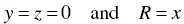

Therefore, Eq. (2.9) becomes

(2.14)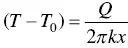

Therefore, the temperature gradient is

(2.15)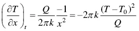

From the above equation and

(2.16)

the cooling rate becomes

(2.17)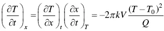

Without preheating the workpiece before welding,

(2.18)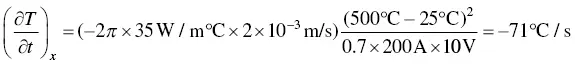

With 250 °C preheating,

(2.19)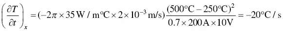

It is clear that the cooling rate is reduced significantly by preheating. Preheating is a common practice in welding high‐strength steels because it reduces the risk of HAZ cracking. In multiple‐pass welding the inter‐pass temperature is equivalent to the preheat temperature T 0in single‐pass welding.

Thus, Eq. (2.17) shows that the cooling rate decreases with increasing Q/V , and Eq. (2.15) shows that the temperature gradient decreases with increasing Q .

Example 2.2Consider 2D ( x , y ) heat flow and 3D ( x , y , z ) heat flow in the workpiece. (a) When heat flow in the workpiece is 2D, does the temperature distribution (including the weld width) change much in the depth direction of the workpiece? (b) What about 3D heat flow? (c) Which equation works better for the thick plate (25 mm thick) in Figure E2.2, and why? (d) How about the thin sheet (3.2 mm thick)? (e) At the same Q and V, how does preheating affect the weld width and cooling rate?