William M. White - Geochemistry
Здесь есть возможность читать онлайн «William M. White - Geochemistry» — ознакомительный отрывок электронной книги совершенно бесплатно, а после прочтения отрывка купить полную версию. В некоторых случаях можно слушать аудио, скачать через торрент в формате fb2 и присутствует краткое содержание. Жанр: unrecognised, на английском языке. Описание произведения, (предисловие) а так же отзывы посетителей доступны на портале библиотеки ЛибКат.
- Название:Geochemistry
- Автор:
- Жанр:
- Год:неизвестен
- ISBN:нет данных
- Рейтинг книги:5 / 5. Голосов: 1
-
Избранное:Добавить в избранное
- Отзывы:
-
Ваша оценка:
Geochemistry: краткое содержание, описание и аннотация
Предлагаем к чтению аннотацию, описание, краткое содержание или предисловие (зависит от того, что написал сам автор книги «Geochemistry»). Если вы не нашли необходимую информацию о книге — напишите в комментариях, мы постараемся отыскать её.
, undergraduate and graduate students will find each of the core principles of geochemistry covered. From defining key principles and methods to examining Earth’s core composition and exploring organic chemistry and fossil fuels, this definitive edition encompasses all the information needed for a solid foundation in the earth sciences for beginners and beyond.
For researchers and applied scientists, this book will act as a useful reference on fundamental theories of geochemistry, applications, and environmental sciences. The new edition includes new chapters on the geochemistry of the Earth’s surface (the “critical zone”), marine geochemistry, and applied geochemistry as it relates to environmental applications and geochemical exploration.
● A review of the fundamentals of geochemical thermodynamics and kinetics, trace element and organic geochemistry
● An introduction to radiogenic and stable isotope geochemistry and applications such as geologic time, ancient climates, and diets of prehistoric people
● Formation of the Earth and composition and origins of the core, the mantle, and the crust
● New chapters that cover soils and streams, the oceans, and geochemistry applied to the environment and mineral exploration
In this foundational look at geochemistry, new learners and professionals will find the answer to the essential principles and techniques of the science behind the Earth and its environs.
Geochemistry — читать онлайн ознакомительный отрывок
Ниже представлен текст книги, разбитый по страницам. Система сохранения места последней прочитанной страницы, позволяет с удобством читать онлайн бесплатно книгу «Geochemistry», без необходимости каждый раз заново искать на чём Вы остановились. Поставьте закладку, и сможете в любой момент перейти на страницу, на которой закончили чтение.
Интервал:
Закладка:
3.2.2 The Gibbs phase rule
The Gibbs ‡phase rule is a rule for determining the degrees of freedom , or variance , of a system at equilibrium . The rule is:
(3.2) 
where ƒ is the degrees of freedom, c is the number of components, and φ is the number of phases. The mathematical analogy is that the degrees of freedom are equal to the number of variables minus the number of equations relating those variables. For example, in a system consisting of just H 2O, if two phases coexist, for example, water and steam, then the system is univariant. Three phases coexist at the triple point of water, so the system is said to be invariant, and T and P are uniquely fixed: there is only one temperature and one pressure at which the three phases of water can coexist (273.15 K and 0.006 MPa). If only one phase is present, for example just liquid water, then we need to specify two variables to describe completely the system. It does not matter which two we pick. We could specify molar volume and temperature and from that we could deduce pressure. Alternatively, we could specify pressure and temperature. There is only one possible value for the molar volume if temperature and pressure are fixed. It is important to remember this applies to intensive parameters. To know volume, an extensive parameter, we would have to fix one additional extensive variable (such as mass or number of moles). And again, we emphasize that all this applies only to systems at equilibrium.
Now consider the hydration of corundum to form gibbsite. There are three phases, but there need be only two components. If these three phases (water, corundum, gibbsite) are at equilibrium, we have only one degree of freedom (i.e., if we know the temperature at which these three phases are in equilibrium, the pressure is also fixed).
Rearranging eqn. 3.2, we also can determine the maximum number of phases that can coexist at equilibrium in any system. The degrees of freedom cannot be less than zero, so for an invariant, one-component system, a maximum of three phases can coexist at equilibrium. In a univariant one-component system, only two phases can coexist. Thus, sillimanite and kyanite can coexist over a range of temperatures, as can kyanite and andalusite, but the three phases of Al 2SiO 5coexist only at one unique temperature and pressure.
Let's consider the example of the three-component system Al 2O 3–H 2O–SiO 2in Figure 3.2. Although many phases are possible in this system, for any given composition of the system only three phases can coexist at equilibrium over a range of temperature and pressure. Four phases (e.g, a, k, s, and p) can coexist only along a one-dimensional line or curve in P–T space. Such points are called univariant lines (or curves). Five phases can coexist at invariant points at which both temperature and pressure are uniquely fixed. Turning this around, if we found a metamorphic rock whose composition fell within the Al 2O 3–H 2O–SiO 2system, and if the rock contained five phases, it would be possible to determine uniquely the temperature and pressure at which the rock equilibrated.
3.2.3 The Clapeyron equation
A common problem in geochemistry is to know how a phase boundary varies in P–T space, for example, how a melting temperature will vary with pressure. At a phase boundary, two phases must be in equilibrium, so Δ G must be 0 for the reaction Phase 1 ⇌ Phase 2. The phase boundary therefore describes the condition:

Thus, the slope of a phase boundary on a temperature-pressure diagram is:
(3.3) 
where ΔV rand ΔS rare the volume and entropy changes associated with the reaction. Equation 3.3is known as the Clausius–Clapeyron equation , or simply the Clapeyron equation . Because ΔV rand ΔS rare functions of temperature and pressure, this is, of course, only an instantaneous slope. For many reactions, however, particularly those involving only solids, the temperature and pressure dependencies of ΔV rand ΔS rwill be small and the Clapeyron slope will be relatively constant over a large T and P range (see Example 3.1).
Because ΔS = ΔH/T , the Clapeyron equation may be equivalently written as:
(3.4) 
Slopes of phase boundaries in P–T space are generally positive, implying that the phases with the largest volumes also generally have the largest entropies (for reasons that become clear from a statistical mechanical treatment). This is particularly true of solid–liquid phase boundaries, although there is one very important exception: water. How do we determine the pressure and temperature dependence of ΔV rand why is ΔV rrelatively T - and P -independent in solids?
We should emphasize that application of the Clapeyron equation is not limited to reactions between two phases in a one-component system but may be applied to any univariant reaction.
Example 3.1The graphite–diamond transition
At 25°C the graphite–diamond transition occurs at 1600 MPa (megapascals, 1 MPa =10 b). Using the standard state (298 K, 0.1 MPa) data below, predict the pressure at which the transformation occurs when temperature is 1000°C.
| Graphite | Diamond | |
| α (K –1) | 1.05 × 10 −05 | 7.50 × 10 −06 |
| β (MPa −1) | 3.08 × 10 −05 | 2.27 × 10 −06 |
| S° (J/K-mol) | 5.74 | 2.38 |
| V (cm 3/mol) | 5.2982 | 3.417 |
Answer: We can use the Clapeyron equation to determine the slope of the phase boundary. Then, assuming that Δ S and Δ V are independent of temperature, we can extrapolate this slope to 1000°C to find the pressure of the phase transition at that temperature.
First, we calculate the volumes of graphite and diamond at 1600 MPa as (eqn. 2.140):
(3.5) 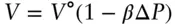
where Δ P is the difference between the pressure of interest (1600 MPa in this case) and the reference pressure (0.1 MPa). Doing so, we find the molar volumes to be 5.037 for graphite and 3.405 for diamond, so Δ V ris −1.6325 cc/mol. The next step will be to calculate Δ S at 1600 MPa. The pressure dependence of entropy is given by equation 2.106: ( ∂S/∂P ) T= − αV . Thus, to determine the effect of pressure we integrate:
(3.6) 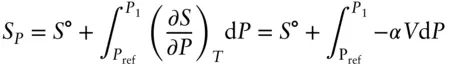
(We use S pto indicate the entropy at the pressure of interest and S° the entropy at the reference pressure.) We need to express V as a function of pressure, so we substitute eqn. 3.5into 3.6:
Читать дальшеИнтервал:
Закладка:
Похожие книги на «Geochemistry»
Представляем Вашему вниманию похожие книги на «Geochemistry» списком для выбора. Мы отобрали схожую по названию и смыслу литературу в надежде предоставить читателям больше вариантов отыскать новые, интересные, ещё непрочитанные произведения.


Обсуждение, отзывы о книге «Geochemistry» и просто собственные мнения читателей. Оставьте ваши комментарии, напишите, что Вы думаете о произведении, его смысле или главных героях. Укажите что конкретно понравилось, а что нет, и почему Вы так считаете.