Philippe J. S. De Brouwer - The Big R-Book
Здесь есть возможность читать онлайн «Philippe J. S. De Brouwer - The Big R-Book» — ознакомительный отрывок электронной книги совершенно бесплатно, а после прочтения отрывка купить полную версию. В некоторых случаях можно слушать аудио, скачать через торрент в формате fb2 и присутствует краткое содержание. Жанр: unrecognised, на английском языке. Описание произведения, (предисловие) а так же отзывы посетителей доступны на портале библиотеки ЛибКат.
- Название:The Big R-Book
- Автор:
- Жанр:
- Год:неизвестен
- ISBN:нет данных
- Рейтинг книги:3 / 5. Голосов: 1
-
Избранное:Добавить в избранное
- Отзывы:
-
Ваша оценка:
The Big R-Book: краткое содержание, описание и аннотация
Предлагаем к чтению аннотацию, описание, краткое содержание или предисловие (зависит от того, что написал сам автор книги «The Big R-Book»). Если вы не нашли необходимую информацию о книге — напишите в комментариях, мы постараемся отыскать её.
The Big R-Book for Professionals: From Data Science to Learning Machines and Reporting with R Provides a practical guide for non-experts with a focus on business users Contains a unique combination of topics including an introduction to R, machine learning, mathematical models, data wrangling, and reporting Uses a practical tone and integrates multiple topics in a coherent framework Demystifies the hype around machine learning and AI by enabling readers to understand the provided models and program them in R Shows readers how to visualize results in static and interactive reports Supplementary materials includes PDF slides based on the book’s content, as well as all the extracted R-code and is available to everyone on a Wiley Book Companion Site
is an excellent guide for science technology, engineering, or mathematics students who wish to make a successful transition from the academic world to the professional. It will also appeal to all young data scientists, quantitative analysts, and analytics professionals, as well as those who make mathematical models.
The Big R-Book — читать онлайн ознакомительный отрывок
Ниже представлен текст книги, разбитый по страницам. Система сохранения места последней прочитанной страницы, позволяет с удобством читать онлайн бесплатно книгу «The Big R-Book», без необходимости каждый раз заново искать на чём Вы остановились. Поставьте закладку, и сможете в любой момент перейти на страницу, на которой закончили чтение.
Интервал:
Закладка:
library(MASS) ## ## Attaching package: ‘MASS’ ## The following object is masked from ‘package:dplyr’:## ##select hist(SP500,col=“khaki3”,freq=FALSE,border=“khaki3”) x <- seq(from= -5,to=5,by=0.001) lines(x, dnorm(x, mean(SP500), sd(SP500)),col=“blue”,lwd=2)
A better way to check for normality is to study the Q-Q plot. A Q-Q plot compares the sample quantiles with the quantiles of the distribution and it makes very clear where deviations appear.
Q-Q plot
library(MASS)
qqnorm(SP500,col=“red”); qqline(SP500,col=“blue”)
From the Q-Q plot in Figure 8.3on page 153 (that is generated by the aforementioned code block), it is clear that the returns of the S&P-500 index are not Normally distributed. Outliers far from the mean appear much more often than the Normal distribution would predict. In other words: returns on stock exchanges have “fat tales.”
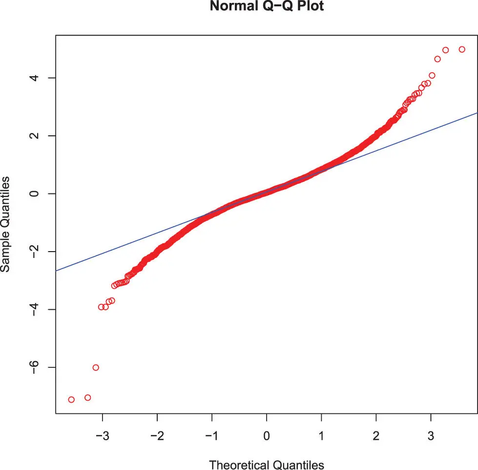
Figure 8.3 : A Q-Q plot is a good way to judge if a set of observations is normally distributed or not.
8.4.2 Binomial Distribution
The Binomial distribution models the probability of an event which has only two possible outcomes. For example, the probability of finding exactly 6 heads in tossing a coin repeatedly for 10 times is estimated during the binomial distribution.
distribution – binomial
The Binomial Distribution in R
As for all distributions, R has four in-built functions to generate binomial distribution:
dbinom(x, size, prob): The density function
dbinom()
pbinom()
dbinom()
pbinom(x, size, prob): The cumulative probability of an event
pbinom()
qbinom(p, size, prob): Gives a number whose cumulative value matches a given probability value
qbinom()
rbinom(n, size, prob): Generates random variables following the binomial distribution.
rbinom()
Following parameters are used:
x: A vector of numbers
p: A vector of probabilities
n: The number of observations
size: The number of trials
prob: The probability of success of each trial
An Example of the Binomial Distribution
The example below illustrates the biniomial distribution and generates the plot in Figure 8.4.
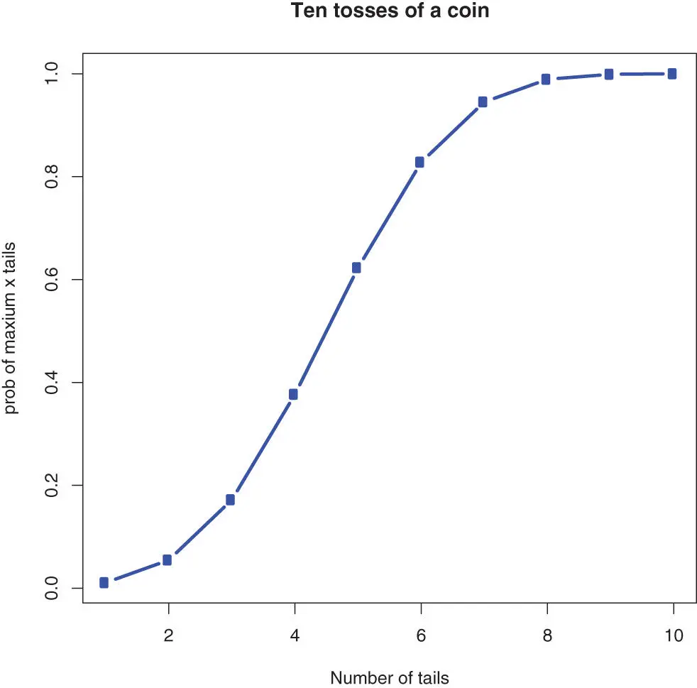
Figure 8.4 : The probability to get maximum x tails when flipping a fair coin, illustrated with the binomial distribution.
# Probability of getting 5 or less heads from 10 tosses of # a coin. pbinom(5,10,0.5) ## [1] 0.6230469 # visualize this for one to 10 numbers of tossesx <-1 :10 y <- pbinom(x,10,0.5) plot(x,y,type=“b”,col=“blue”, lwd=3, xlab=“Number of tails”, ylab=“prob of maxium x tails”, main=“Ten tosses of a coin”) # How many heads should we at least expect (with a probability # of 0.25) when a coin is tossed 10 times. qbinom(0.25,10,1 /2) ## [1] 4
Similar to theNormal distribution, random draws of the Binomial distribution can be obtained via a function that starts with the letter ‘r’: rbinom().
rbinom()
# Find 20 random numbers of tails from and event of 10 tosses # of a coin rbinom(20,10,.5) ## [1] 5 7 2 6 7 4 6 7 3 2 5 9 5 9 5 5 5 5 5 6
8.5. Creating an Overview of Data Characteristics
In the Chapter 4 “The Basics of R” on page 21, we presented some of the basic functions of R that – of course – include the some of the most important functions to describe data (such as mean and standard deviation).
Mileage may vary, but in many research people want to document what they have done and will need to include some summary statistics in their paper or model documentation. The standard summaryof the relevant object might be sufficient.
N <-100 t <- data.frame(id = 1 :N, result = rnorm(N)) summary(t) ## id result ## Min. : 1.00 Min. :-1.8278 ## 1st Qu.: 25.75 1st Qu.:-0.5888 ## Median : 50.50 Median :-0.0487 ## Mean : 50.50 Mean :-0.0252 ## 3rd Qu.: 75.25 3rd Qu.: 0.4902 ## Max. :100.00 Max. : 2.3215
This already produces a neat summary that can directly be used in most reports. 2
 Note – A tibble is a special form of data-frame
A tibble and data frame will produce the same summaries.
We might want to produce some specific information that somehow follows the format of the table. To illustrate this, we start from the dataset mtcarsand assume that we want to make a summary per brand for the top-brands (defined as the most frequent appearing in our database).
library(tidyverse) # not only for %>% but also for group_by, etc. # In mtcars the type of the car is only in the column names, # so we need to extract it to add it to the datan <- rownames(mtcars) # Now, add a column brand (use the first letters of the type)t <-mtcars %>% mutate(brand = str_sub(n, 1, 4)) # add column
To achieve this, the function group_by()from dplyrwill be very handy. Note that this function does not change the dataset as such, it rather adds a layer of information about the grouping.
group_by()
# First, we need to find out which are the most abundant brands # in our dataset (set cutoff at 2: at least 2 cars in database)top_brands <- count(t, brand) %>% filter(n >=2) # top_brands is not simplified to a vector in the tidyverse print(top_brands) ## # A tibble: 5 x 2 ## brand n
Table 8.2: Summary information based on the dataset mtcars.
| brand | avgDSP | avgCYL | minMPG | medMPG | avgMPG | maxMPG |
| Fiat | 78.9 | 4.0 | 27.3 | 29.85 | 29.85 | 32.4 |
| Horn | 309.0 | 7.0 | 18.7 | 20.05 | 20.05 | 21.4 |
| Mazd | 160.0 | 6.0 | 21.0 | 21.00 | 21.00 | 21.0 |
| Merc | 207.2 | 6.3 | 15.2 | 17.80 | 19.01 | 24.4 |
| Toyo | 95.6 | 4.0 | 21.5 | 27.70 | 27.70 | 33.9 |
## ## 1 Fiat 2 ## 2 Horn 2 ## 3 Mazd 2 ## 4 Merc 7 ## 5 Toyo 2 grouped_cars <-t %>% # start with cars filter(brand %in%top_brands $brand) %>% # only top-brands group_by(brand) %>% summarise( avgDSP = round( mean(disp), 1), avgCYL = round( mean(cyl), 1), minMPG = min(mpg), medMPG = median(mpg), avgMPG = round( mean(mpg),2), maxMPG = max(mpg), ) print(grouped_cars) ## # A tibble: 5 x 7 ## brand avgDSP avgCYL minMPG medMPGavgMPGmaxMPG ## ## 1 Fiat 78.8 4 27.3 29.8 29.8 32.4 ## 2 Horn 309 7 18.7 20.0 20.0 21.4 ## 3 Mazd 160 6 21 21 21 21 ## 4 Merc 207. 6.3 15.2 17.8 19.0 24.4 ## 5 Toyo 95.6 4 21.5 27.7 27.7 33.9
Читать дальшеИнтервал:
Закладка:
Похожие книги на «The Big R-Book»
Представляем Вашему вниманию похожие книги на «The Big R-Book» списком для выбора. Мы отобрали схожую по названию и смыслу литературу в надежде предоставить читателям больше вариантов отыскать новые, интересные, ещё непрочитанные произведения.


Обсуждение, отзывы о книге «The Big R-Book» и просто собственные мнения читателей. Оставьте ваши комментарии, напишите, что Вы думаете о произведении, его смысле или главных героях. Укажите что конкретно понравилось, а что нет, и почему Вы так считаете.