Philippe J. S. De Brouwer - The Big R-Book

Note that the original meaning of “x” is gone.

We recommend to use this pipe operator only when no confusion is possible. We also argue that this pipe operator makes code less readable, while not really making the code shorter.

When you come from a background of compiled languages that provides fine graded control over memory management (such as C or C++), you might not directly see the need for pipes that much. However, it does reduce the amount of text that needs to be typed and makes the code more readable.

Indeed, the piping operator will not provide a speed increase nor memory advantage even if we would create a new variable at every line. R has a pretty good memory management and it does only copy columns when they are really modified. For example, have a careful look at the following:

library(pryr) x <- runif(100) object_size(x) ## 840 B y <-x # x and y together do not take more memory than only x. object_size(x,y) ## 840 B y <-y *2 # Now, they are different and are stored separately in memory. object_size(x,y) ## 1.68 kB

The piping operator can be confusing at first and is not really necessary (unless to read code that is using it). However, it has the advantage to make code more readable – once used to it – and it also makes code shorter. Finally, it allows the reader of the code to focus more on what is going on (the actions instead of the data, since that is passed over invisibly).

Pipes are as spices in the kitchen. Use them, but do so with moderation. A good rule of thumb is that five lines is enough, and simple one-line commands do not need to be broken down in more lines in order to use a pipe.

1 1According to the Tiobe-index (see https://www.tiobe.com/tiobe-index), R is the 14th most popular programming language and still on the rise.

2 2More information can be found in this article of Hadley Wickham: https://tidyverse.tidyverse.org/articles/manifesto.html.

3 3A notable exception here is ggplot2 This package uses operator overloading instead of piping (overloading of the + operator).

4 4Here we use the notation package1::function1() to make clear that the function1 is the one as defined in package1.

5 5The standard functions to read in data are covered in Section 4.8 “Selected Data Interfaces” on page 75.

6 6Rectangular data is data that – when printed – looks like a rectangle, for example movies and pictures are not rectangular data, while a CSV file or a database table are rectangular data.

7 7Categorical variables are variables that have a fixed and known set of possible values. These values might or might not have a (strict) order relation. For example, “sex” (M or F) would not have an order, but salary brackets might have.

8 8Of course, if you need something else you will want to use the package that does exactly what you want. Here are some good ones that adhere largely to the tidyverse philosophy: jsonlite for JSON, xml2 for XML, httr for web APIs, rvest for web scraping, DBI for relational databases—a good resources is http://db.rstudio.com.

9 9The lack of coherent support for the modelling and reporting area makes clear that the tidyverse is not yet a candidate to service the whole development cycle of the company yet. Modelling departments might want to have a look at the tidymodels package.tidymodels

10 10This quote is generally attributed to the Voltaire (pen-name of Jean-Marie Arouet; 1694–1778) and is published in the French National Convention of 8 May, 1793 (see con (1793) – page 72). After that many leaders and writers of comic books have used many variants of this phrase.

11 11R's piping operator is very similar to the piping command that youmight know fromthe most of the CLI shells of popular *nix systems where messages like the following can go a long way: dmesg | grep “Bluetooth”, though differences will appear in more complicated commands.

12 12The function lm() generates a linear model in R of the form . More information can be found in Section 21.1 “Linear Regression” on page 375. The functions summary() and coefficients() that are used on the following pages are also explained there.

statistics

Ameasure of central tendency is a single value that attempts to describe a set of data by identifying the central position within that set of data. As such, measures of central tendency are sometimes called measures of central location. They are also classed as summary statistics. The mean (often called the average) is most likely the measure of central tendency that you are most familiar with, but there are others, such as the median and the mode.

central tendency

measure – central tendency

The mean, median, and mode are all valid measures of central tendency, but under different conditions, some measures of central tendency become more appropriate to use than others. In the following sections, we will look at the mean, mode, and median, and learn how to calculate them and under what conditions they are most appropriate to be used.

mean

Probably the most used measure of central tendency is the “mean.” In this section we will start from the arithmetic mean, but illustrate some other concepts that might be more suited in some situations too.

central tendency – mean

mean – arithmetic

The most popular type of mean is the “arithmetic mean.” It is the average of a set of numerical values; and it is calculated by adding those values first together and then dividing by the number of values in the aforementioned set.

mean – arithmetic

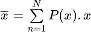(for discrete distributions)

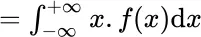(for continuous distributions)

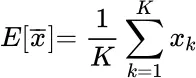
The unbiased estimator of the mean for K observations x kis:

mean

P()

probability

probability

f()

Not surprisingly, the arithmetic mean in R is calculated by the function mean().

probability density function