Philippe J. S. De Brouwer - The Big R-Book

mean()

This is a dispatcher function 1 and it will work in a meaningful way for a variety of objects, such as vectors, matrices, etc.

# The mean of a vector:x <- c(1,2,3,4,5,60) mean(x) ## [1] 12.5 # Missing values will block the override the result:x <- c(1,2,3,4,5,60,NA) mean(x) ## [1] NA # Missing values can be ignored with na.rm = TRUE: mean(x, na.rm = TRUE) ## [1] 12.5 # This works also for a matrix:M <- matrix( c(1,2,3,4,5,60), nrow=3) mean(M) ## [1] 12.5

The mean is highly influenced by the outliers. To mitigate this to some extend the parameter trimallows to remove the tails. It will sort all values and then remove the x% smallest and x% largest observations.

v <- c(1,2,3,4,5,6000) mean(v) ## [1] 1002.5 mean(v, trim = 0.2) ## [1] 3.5

mean – generalized

More generally, a mean can be defined as follows:

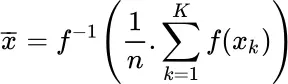
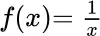
Popular choices for f()are:

f ( x ) = x : arithmetic mean,

: harmonic mean,

f ( x ) = x m: power mean,

f ( x ) = ln x : geometric mean,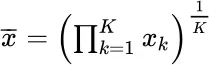

arithmetic mean

mean – harmonic

harmonic mean

mean – power

power mean

mean – geometric

geometric mean

One particular generalized mean is the power mean or Hölder mean. It is defined for a set of K positive numbers x kby

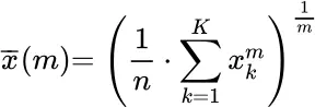
holder mean

mean – holder

by choosing particular values for m one can get the quadratic, arithmetic, geometric and harmonic means.

mean – quadratic

m → ∞: maximum of x k

m = 2: quadratic mean

m = 1: arithmetic mean

m → 0: geometric mean

m = 1: harmonic mean

m → −∞: minimum of x k

What is the average return when you know that the share price had the following returns: −50%, +50%,−50%, +50%. Try the arithmetic mean and the mean of the log-returns.

returns <- c(0.5, -0.5,0.5, -0.5) # Arithmetic mean:aritmean <- mean(returns) # The ln-mean:log_returns <-returns for(k in1 :length(returns)) { log_returns[k] <- log( returns[k] +1) } logmean <- mean(log_returns) exp(logmean) -1 ## [1] -0.1339746 # What is the value of the investment after these returns:V_0 <-1 V_T <-V_0 for(k in1 :length(returns)) { V_T <-V_T *(returns[k] +1) } V_T ## [1] 0.5625 # Compare this to our predictions: ## mean of log-returnsV_0 *( exp(logmean) -1) ## [1] -0.1339746 ## mean of returnsV_0 *(aritmean +1) ## [1] 1

median

While the mean (and the average in particular) is widely used, it is actually quite vulnerable to outliers. It would therefore, make sense to have a measure that is less influenced by the outliers and rather answers the question: what would a typical observation look like. The median is such measure.

central tendency – median

The median is the middle-value so that 50% of the observations are lower and 50% are higher.

x <- c(1 :5,5e10,NA) x ## [1] 1e+00 2e+00 3e+00 4e+00 5e+00 5e+10 NA median(x) # no meaningful result with NAs## [1] NA median(x,na.rm = TRUE) # ignore the NA## [1] 3.5 # Note how the median is not impacted by the outlier, # but the outlier dominates the mean: mean(x, na.rm = TRUE) ## [1] 8333333336

mode

central tendency – mode

The mode is the value that has highest probability to occur. For a series of observations, this should be the one that occurs most often. Note that the mode is also defined for variables that have no order-relation (even labels such as “green,” “yellow,” etc. have amode, but not a mean or median—without further abstraction or a numerical representation).

In R, the function mode()or storage.mode()returns a character string describing how a variable is stored. In fact, R does not have a standard function to calculate mode, so let us create our own:

mode()

storage.mode()

# my_mode # Finds the first mode (only one) # Arguments: # v -- numeric vector or factor # Returns: # the first modemy_mode <- function(v) { uniqv <- unique(v) tabv <- tabulate( match(v, uniqv)) uniqv[ which.max(tabv)] } # now test this functionx <- c(1,2,3,3,4,5,60,NA) my_mode(x) ## [1] 3 x1 <- c(“relevant”, “N/A”, “undesired”, “great”, “N/A”, “undesired”, “great”, “great”) my_mode(x1) ## [1] “great” # text from https://www.r-project.org/about.htmlt <-“R is available as Free Software under the terms of the Free Software Foundation’s GNU General Public License in source code form. It compiles and runs on a wide variety of UNIX platforms and similar systems (including FreeBSD and Linux), Windows and MacOS.” v <- unlist( strsplit(t,split=” “)) my_mode(v) ## [1] “and”

unique()

Linux

FreeBSD

tabulate()

uniqv()

While this function works fine on the examples provided, it only returns the first mode encountered. In general, however, the mode is not necessarily unique and it might make sense to return them all. This can be done by modifying the code as follows: