Philippe J. S. De Brouwer - The Big R-Book
Здесь есть возможность читать онлайн «Philippe J. S. De Brouwer - The Big R-Book» — ознакомительный отрывок электронной книги совершенно бесплатно, а после прочтения отрывка купить полную версию. В некоторых случаях можно слушать аудио, скачать через торрент в формате fb2 и присутствует краткое содержание. Жанр: unrecognised, на английском языке. Описание произведения, (предисловие) а так же отзывы посетителей доступны на портале библиотеки ЛибКат.

- Название:The Big R-Book
- Автор:
- Жанр:
- Год:неизвестен
- ISBN:нет данных
- Рейтинг книги:3 / 5. Голосов: 1
-
Избранное:Добавить в избранное
- Отзывы:
-
Ваша оценка:
The Big R-Book: краткое содержание, описание и аннотация
Предлагаем к чтению аннотацию, описание, краткое содержание или предисловие (зависит от того, что написал сам автор книги «The Big R-Book»). Если вы не нашли необходимую информацию о книге — напишите в комментариях, мы постараемся отыскать её.
The Big R-Book for Professionals: From Data Science to Learning Machines and Reporting with R Provides a practical guide for non-experts with a focus on business users Contains a unique combination of topics including an introduction to R, machine learning, mathematical models, data wrangling, and reporting Uses a practical tone and integrates multiple topics in a coherent framework Demystifies the hype around machine learning and AI by enabling readers to understand the provided models and program them in R Shows readers how to visualize results in static and interactive reports Supplementary materials includes PDF slides based on the book’s content, as well as all the extracted R-code and is available to everyone on a Wiley Book Companion Site
is an excellent guide for science technology, engineering, or mathematics students who wish to make a successful transition from the academic world to the professional. It will also appeal to all young data scientists, quantitative analysts, and analytics professionals, as well as those who make mathematical models.
The Big R-Book — читать онлайн ознакомительный отрывок
Ниже представлен текст книги, разбитый по страницам. Система сохранения места последней прочитанной страницы, позволяет с удобством читать онлайн бесплатно книгу «The Big R-Book», без необходимости каждый раз заново искать на чём Вы остановились. Поставьте закладку, и сможете в любой момент перейти на страницу, на которой закончили чтение.
Интервал:
Закладка:
1 x = c(1, 2, 33, 44) and y = c(22, 23, 100, 200),
2 x = c(1 : 10) and y = 2 * x,
3 x = c(1 : 10) and y = exp(x),
Plot y in function of x . What is their Pearson correlation? What is their Spearman correlation? How do you understand that?
 Warning – Correlation is more specific than relation
Not even the Spearman correlation will discover all types of dependencies. Consider the example above with x 2.
x <- c( -10 :10) cor( rank(x), rank(x ∧2)) ## [1] 0
8.3.3 Chi-square Tests
Chi-square test is a statistical method to determine if two categorical variables have a significant correlation between them. Both those variables should be from same population, and they should be categorical like “Yes/No,” “Male/Female,” “Red/Amber/Green,” etc.
test – chi square
For example, we can build a dataset with observations on people’s ice-cream buying pattern and try to correlate the gender of a person with the flavour of the ice-cream they prefer. If a correlation is found, we can plan for appropriate stock of flavours by knowing the number of gender of people visiting.
Chi-Square test in R
Function use for chisq.test()
chisq.test(data)
where datais the data in form of a table containing the count value of the variables
For example, we can use the mtcarsdataset that is most probably loaded when R was initialised.
# we use the dataset mtcars from MASSdf <- data.frame(mtcars $cyl,mtcars $am) chisq.test(df) ## Warning in chisq.test(df): Chi-squared approximation may be incorrect ## ## Pearson’s Chi-squared test ## ## data: df ## X-squared = 25.077, df = 31, p-value = 0.7643
chisq.test()
The chi-square test reports a p-value. This p-value is the probability that the correlations is actually insignificant. It appears that in practice a correlation lower than 5% can be considered as insignificant. In this example, the p-value is higher than 0.05, so there is no significant correlation.
8.4. Distributions
R is a statistical language and most of thework in R will include statistics. Therefore we introduce the reader to how statistical distributions are implemented in R and how they can be used.
The names of the functions related to statistical distributions in R are composed of two sections: the first letter refers to the function (in the following) and the remainder is the distribution name.
d: The pdf (probability density function)
p: The cdf (cumulative probability density function)
q: The quantile function
r: The random number generator.
probability density function
cdf
cumulative density function
quantile function
random
distribution – normal
distribution – exponential
distribution – log-normal
distribution – logistic
distribution – geometric
distribution – Poisson
distribution – t
distribution – f
distribution – beta
distribution – weibull
distribution – binomial
distribution – negative
binomial
distribution – chi-squared
distribution – uniform
distribution – gamma
distribution – cauchy
distribution – hypergeometric
Table 8.1: Common distributions and their names in R .
| Distribution | R-name | Distribution | R-name |
| Normal | norm | Weibull | weibull |
| Exponential exp | Binomial | binom | |
| Log-normal | lnorm | Negative binomial | nbinom |
| Logistic | logis | χ 2 | chisq |
| Geometric | geom | Uniform | unif |
| Poisson | pois | Gamma | gamma |
| t | t | Cauchy | cauchy |
| f | f | Hypergeometric | hyper |
| Beta | beta |
As all distributions work in a very similar way, we use the normal distribution to show how the logic works.
8.4.1 Normal Distribution
distribution – normal
One of the most quintessential distributions is the Gaussian distribution or Normal distribution. Its probability density function resembles a bell. The centre of the curve is the mean of the data set. In the graph, 50% of values lie to the left of the mean and the other 50% lie to the right of the graph.
The Normal Distribution in R
R has four built-in functions to work with the normal distribution. They are described below.
dnorm(x, mean, sd): The height of the probability distribution
pnorm(x, mean, sd): The cumulative distribution function (the probability of the observation to be lower than x)
dnorm()
pnorm()
qnorm(p, mean, sd): Gives a number whose cumulative value matches the given probability value p
rnorm(n, mean, sd): Generates normally distributed variables,
qnorm()
rnorm()
with
x: A vector of numbers
p: A vector of probabilities
n: The number of observations(sample size)
mean: The mean value of the sample data (default is zero)
sd: The standard deviation (default is 1).
Illustrating the Normal Distribution
In the following example we generate data with the random generator function rnorm()and then compare the histogramof that data with the ideal probability density function of the Normal distribution. The output of the following code is Figure 8.1on this page.
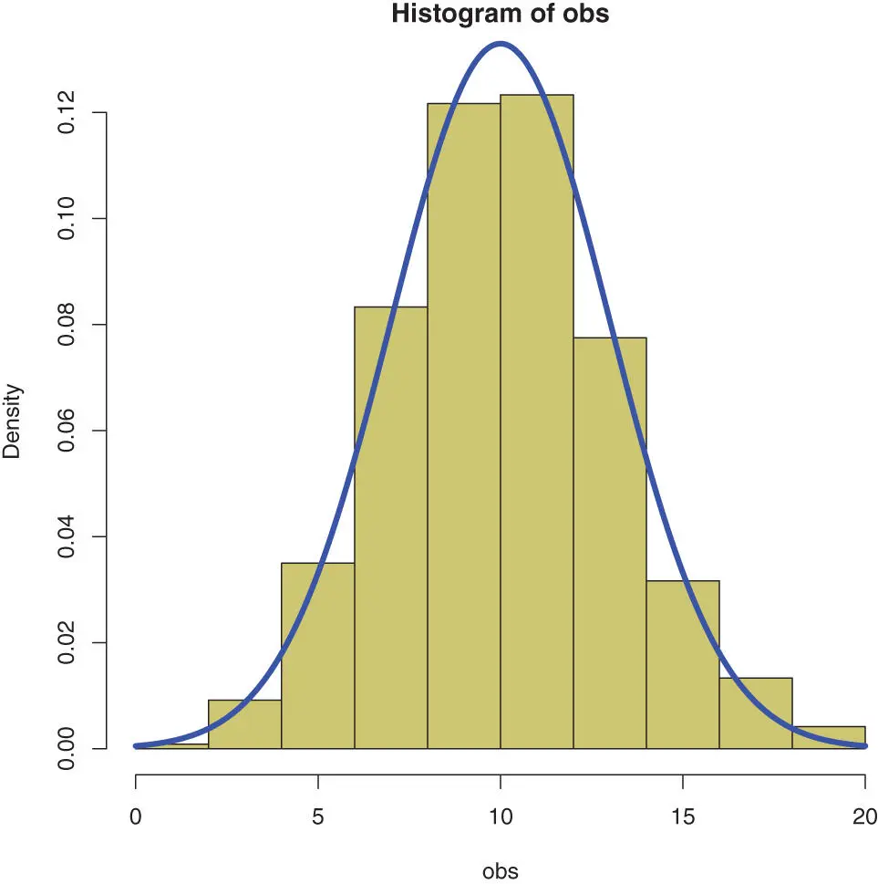
Figure 8.1 : A comparison between a set of random numbers drawn from the normal distribution (khaki) and the theoretical shape of the normal distribution in blue.
obs <- rnorm(600,10,3) hist(obs,col=“khaki3”,freq=FALSE) x <- seq(from=,to=20,by=0.001) lines(x, dnorm(x,10,3),col=“blue”,lwd=4)
Case Study: Returns on the Stock Exchange
In this simple illustration, we will compare the returns of the index S&P500 to the Normal distribution. The output of the following code is Figure 8.2on this page.
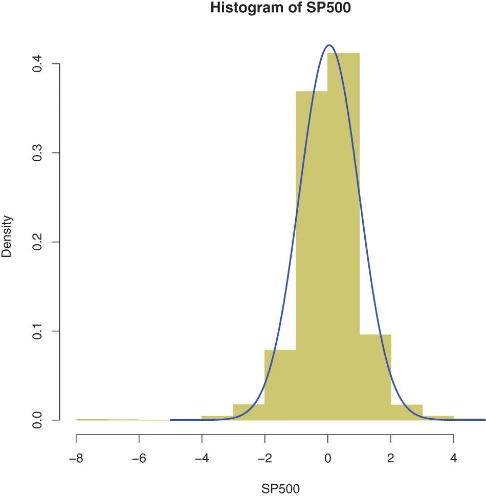
Figure 8.2 : The same plot for the returns of the SP500 index seems acceptable, though there are outliers (where the normal distribution converges fast to zero).
Читать дальшеИнтервал:
Закладка:
Похожие книги на «The Big R-Book»
Представляем Вашему вниманию похожие книги на «The Big R-Book» списком для выбора. Мы отобрали схожую по названию и смыслу литературу в надежде предоставить читателям больше вариантов отыскать новые, интересные, ещё непрочитанные произведения.


Обсуждение, отзывы о книге «The Big R-Book» и просто собственные мнения читателей. Оставьте ваши комментарии, напишите, что Вы думаете о произведении, его смысле или главных героях. Укажите что конкретно понравилось, а что нет, и почему Вы так считаете.