Philippe J. S. De Brouwer - The Big R-Book

try()

tryCatch()

handler

# f1 # Dummy function that from which only the error throwing part0 # is shown.f1 <- function() { # Here goes the long code that might be doing something risky # (e.g. connecting to a database, uploading file, etc.) # and finally, if it goes wrong: stop(“Early exit from f1!”) # throw error} tryCatch( f1(), # the function to tryerror = function(e) { paste(“_ERROR_:”,e)}, warning = function(w) { paste(“_WARNING_:”,w)}, message = function(m) { paste(“_MESSSAGE_:”,m)}, finally=“Last command” # do at the end) ## [1] “_ERROR_: Error in f1(): Early exit from f1!\n”

As can be understood from the example above, the error handler should not be evaluated if f1 does not throw an error. That is why they use error handling. So the following will not work:

# f1 # Dummy function that from which only the error throwing part # is shown.f1 <- function() { # Here goes the long code that might be doing something risky # (e.g. connecting to a database, uploading file, etc.) # and finally, if it goes wrong: stop(“Early exit from f1!”) # something went wrong} %>% tryCatch( error = function(e) { paste(“_ERROR_:”,e)}, warning = function(w) { paste(“_WARNING_:”,w)}, message = function(m) { paste(“_MESSSAGE_:”,m)}, finally=“Last command” # do at the end) # Note that it fails in silence.

There is a lot more to error catching than meets the eye here. We recommend to read the documentation of the relevant functions carefully. Another good place to start is “Advanced R,” page 163, Wickham (2014).

Another issue when using the pipe operator %>%occurs when functions use explicitely the current environment. In those functions, one will have to be explicit which environment to use. More about environments and scoping can be found in Chapter 5on page 81.

Below we create random data that has a linear dependency and try to fit a linear model on that data. 12

# This will not work, because lm() is not designed for the pipe.lm1 <- tibble(“x” = runif(10)) %>% within(y <-2 *x +4 + rnorm(10, mean=0, sd=0.5)) %>% lm(y ~x) ## Error in as.data.frame.default(data): cannot coerce class ““formula”” to a data.frame

The aforementioned code fails. This is because R will not automatically add something like data = tand use the “t” as far as defined till the line before. The function lm()expects as first argument the formula, where the pipe command would put the data in the first argument. Therefore, magrittrprovides a special pipe operator that basically passes on the variables of the data frame of the line before, so that they can be addressed directly: the %$%.

# The Tidyverse only makes the %>% pipe available. So, to use the # special pipes, we need to load magrittr library(magrittr) ## ## Attaching package: ‘magrittr’ ## The following object is masked from ‘package:purrr’: ## ## set_names ## The following object is masked from ‘package:tidyr’: ## ## extract lm2 <- tibble(“x” = runif(10)) %>% within(y <-2 *x +4 + rnorm(10, mean=0,sd=0.5)) %$% lm(y ~x) summary(lm2) ## ## Call: ## lm(formula = y ~ x) ## ## Residuals: ## Min 1Q Median 3Q Max ## -0.6101 -0.3534 -0.1390 0.2685 0.8798 ## ## Coefficients: ## Estimate Std. Error t value Pr(>|t|) ## (Intercept) 4.0770 0.3109 13.115 1.09e-06 *** ## x 2.2068 0.5308 4.158 0.00317 ** ## --- ## Signif. codes: ## 0 ‘***’ 0.001 ‘**’ 0.01 ‘*’ 0.05 ‘.’ 0.1 ‘ ’ 1 ## ## Residual standard error: 0.5171 on 8 degrees of freedom ## Multiple R-squared: 0.6836,Adjusted R-squared: 0.6441 ## F-statistic: 17.29 on 1 and 8 DF, p-value: 0.003174

This can be elaborated further:

coeff <- tibble(“x” = runif(10)) %>% within(y <-2 *x +4 + rnorm(10, mean=0,sd=0.5)) %$% lm(y ~x) %>%summary %>%coefficients coeff ## Estimate Std. Error t value Pr(>|t|) ## (Intercept) 4.131934 0.2077024 19.893534 4.248422e-08 ## x 1.743997 0.3390430 5.143882 8.809194e-04

Note how we can omit the brackets for functions that do not take any argument.

This works nice, but now imagine that we want to keep “t” as the tibble, but still add some operations on it – for example plot it. In that case, there is the special %T>%“T-pipe” that will rather pass on the left side of the expression than the right side. The output of the code below is the plot in Figure 7.3on page 136.

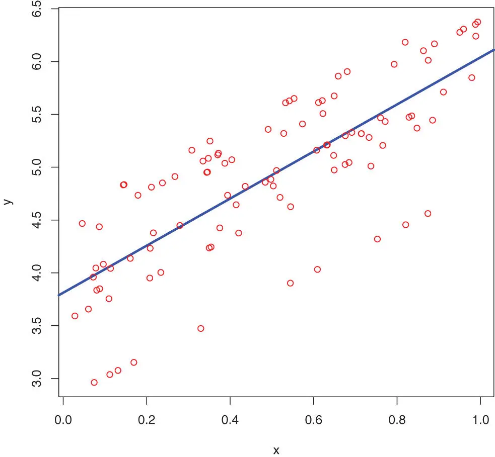
Figure 7.3: A linear model fit on generated data to illustrate the piping command.

library(magrittr) t <- tibble(“x” = runif(100)) %>% within(y <-2 *x +4 + rnorm(10, mean=0, sd=0.5)) %T>% plot(col=“red”) # The function plot does not return anything # so we used the %T>% pipe.lm3 <-t %$% lm(y ~x) %T>% # pass on the linear modelsummary %T>% # further pass on the linear modelcoefficients tcoef <-lm3 %>%coefficients # we anyhow need the coefficients # Add the model (the solid line) to the previous plot: abline(a = tcoef[1], b=tcoef[2], col=“blue”, lwd=3)

This last variation of the pipe operator allows us to simplify the first line, by providing an assignment with a special piping operator.

x <- c(1,2,3) # The following line:x <-x %>%mean # is equivalent with the following:x %<>%mean # Show x:x ## [1] 2