Philippe J. S. De Brouwer - The Big R-Book
Здесь есть возможность читать онлайн «Philippe J. S. De Brouwer - The Big R-Book» — ознакомительный отрывок электронной книги совершенно бесплатно, а после прочтения отрывка купить полную версию. В некоторых случаях можно слушать аудио, скачать через торрент в формате fb2 и присутствует краткое содержание. Жанр: unrecognised, на английском языке. Описание произведения, (предисловие) а так же отзывы посетителей доступны на портале библиотеки ЛибКат.
- Название:The Big R-Book
- Автор:
- Жанр:
- Год:неизвестен
- ISBN:нет данных
- Рейтинг книги:3 / 5. Голосов: 1
-
Избранное:Добавить в избранное
- Отзывы:
-
Ваша оценка:
The Big R-Book: краткое содержание, описание и аннотация
Предлагаем к чтению аннотацию, описание, краткое содержание или предисловие (зависит от того, что написал сам автор книги «The Big R-Book»). Если вы не нашли необходимую информацию о книге — напишите в комментариях, мы постараемся отыскать её.
The Big R-Book for Professionals: From Data Science to Learning Machines and Reporting with R Provides a practical guide for non-experts with a focus on business users Contains a unique combination of topics including an introduction to R, machine learning, mathematical models, data wrangling, and reporting Uses a practical tone and integrates multiple topics in a coherent framework Demystifies the hype around machine learning and AI by enabling readers to understand the provided models and program them in R Shows readers how to visualize results in static and interactive reports Supplementary materials includes PDF slides based on the book’s content, as well as all the extracted R-code and is available to everyone on a Wiley Book Companion Site
is an excellent guide for science technology, engineering, or mathematics students who wish to make a successful transition from the academic world to the professional. It will also appeal to all young data scientists, quantitative analysts, and analytics professionals, as well as those who make mathematical models.
The Big R-Book — читать онлайн ознакомительный отрывок
Ниже представлен текст книги, разбитый по страницам. Система сохранения места последней прочитанной страницы, позволяет с удобством читать онлайн бесплатно книгу «The Big R-Book», без необходимости каждый раз заново искать на чём Вы остановились. Поставьте закладку, и сможете в любой момент перейти на страницу, на которой закончили чтение.
Интервал:
Закладка:
# my_mode # Finds the mode(s) of a vector v # Arguments: # v -- numeric vector or factor # return.all -- boolean -- set to true to return all modes # Returns: # the modal elementsmy_mode <- function(v, return.all = FALSE) { uniqv <- unique(v) tabv <- tabulate( match(v, uniqv)) if(return.all) { uniqv[tabv == max(tabv)] } else{ uniqv[ which.max(tabv)] } } # example:x <- c(1,2,2,3,3,4,5) my_mode(x) ## [1] 2 my_mode(x, return.all = TRUE) ## [1] 2 3
 Hint – Use default values to keep code backwards compatible
We were confident that it was fine to over-ride the definition of the function my_mode. Indeed, if the function was already used in some older code, then one would expect to see only one mode appear. That behaviour is still the same, because we chose the default value for the optional parameter return.allto be FALSE. If the default choice would be TRUE, then older code would produce wrong results and if we would not use a default value, then older code would fail to run.
8.2. Measures of Variation or Spread
measures of spread
Variation or spread measures how different observations are compared to the mean or other central measure. If variation is small, one can expect observations to be closer to each other.
Definition: Variance
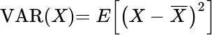
variance
8.2.1 Standard Deviation
Definition: Standard deviation
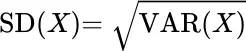
spread – standard deviation
standard deviation
The estimator for standard deviation is:

t <- rnorm(100, mean=, sd=20) var(t) ## [1] 248.2647 sd(t) ## [1] 15.75642 sqrt( var(t)) ## [1] 15.75642 sqrt( sum((t - mean(t)) ∧2) /( length(t) -1)) ## [1] 15.75642
sd()
8.2.2 Median absolute deviation
Definition: mad
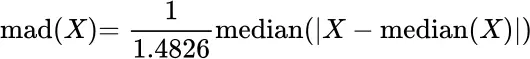
mad
median absolute deviation
mad(t) ## [1] 14.54922 mad(t,constant=1) ## [1] 9.813314
mad()
The default “constant=1.4826” (approximately 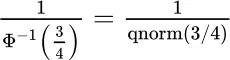 ensures consistency, i.e.,

for X idistributed as N( μ , σ 2) and large n.
8.3. Measures of Covariation
covariation
When there is more than one variable, it is useful to understand what the interdependencies of variables are. For example when measuring the size of peoples hands and their length, one can expect that people with larger hands on average are taller than people with smaller hands. The hand size and length are positively correlated.
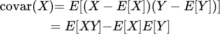
The basic measure for linear interdependence is covariance, defined as
8.3.1 8.3.1 The Pearson Correlation
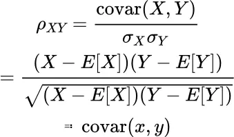
An important metric for linear relationship is the Pearson correlation coefficient ρ .
correlation – Pearson
Definition: Pearson Correlation Coefficient
cor(mtcars $hp,mtcars $wt) ## [1] 0.6587479
cor()
Of course, we also have functions that provide the covariance matrix and functions that convert the one in the other.
d <- data.frame(mpg = mtcars $mpg, wt = mtcars $wt, hp = mtcars $hp) # Note that we can feed a whole data-frame in the functions. var(d) ## mpg wt hp ## mpg 36.324103 -5.116685 -320.73206 ## wt -5.116685 0. 957379 44.19266 ## hp -320.732056 44.192661 4700.86694 cov(d) ## mpg wt hp ## mpg 36.324103 -5.116685 -320.73206 ## wt -5.116685 0.957379 44.19266 ## hp -320.732056 44.192661 4700.86694 cor(d) ## mpg wt hp ## mpg 1.0000000 -0.8676594 -0.7761684 ## wt -0.8676594 1.0000000 0.6587479 ## hp -0.7761684 0.6587479 1.0000000
var()
cov()
cor()
cov2cor( cov(d)) ## mpg wt hp ## mpg 1.0000000 -0.8676594 -0.7761684 ## wt -0.8676594 1.0000000 0.6587479 ## hp -0.7761684 0.6587479 1.0000000
cov2cor()
8.3.2 8.3.2 The Spearman Correlation
The measure for correlation, as defined in previous section, actually tests for a linear relation. This means that even the presence of a strong non-linear relationship can go undetected.
x <- c( -10 :10) df <- data.frame(x=x, x_sq=x ∧2, x_abs= abs(x), x_exp= exp(x)) cor(df) ## x x_sq x_abs x_exp ## x 1.000000 0.0000000 0.0000000 0.5271730 ## x_sq 0.000000 1.0000000 0.9671773 0.5491490 ## x_abs 0.000000 0.9671773 1.0000000 0.4663645 ## x_exp 0.527173 0.5491490 0.4663645 1.0000000
The correlation between x and x 2is zero, and the correlation between x and exp ( x ) is a meagre 0.527173.
correlation – Spearman
The Spearman correlation is the correlation applied to the ranks of the data. It is one if an increase in the variable X is always accompanied with an increase in variable Y .
cor(rank(df$x), rank(df$x_exp)) ## [1] 1
The Spearman correlation checks for a relationship that can bemore general than only linear. It will be one if X increases when Y increases.
 Question #10
Consider the vectors
Читать дальшеИнтервал:
Закладка:
Похожие книги на «The Big R-Book»
Представляем Вашему вниманию похожие книги на «The Big R-Book» списком для выбора. Мы отобрали схожую по названию и смыслу литературу в надежде предоставить читателям больше вариантов отыскать новые, интересные, ещё непрочитанные произведения.


Обсуждение, отзывы о книге «The Big R-Book» и просто собственные мнения читателей. Оставьте ваши комментарии, напишите, что Вы думаете о произведении, его смысле или главных героях. Укажите что конкретно понравилось, а что нет, и почему Вы так считаете.