Robert Bartoszynski - Probability and Statistical Inference

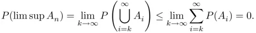
Paraphrasing the assertion of the lemma, if probabilities of events decrease to zero fast enough to make the series converge, then with probability 1 only finitely many among events will occur. We will prove the converse (under an additional assumption), known as the second Borel–Cantelli lemma, in Chapter 4.

In the remainder of this section, we will discuss some theoretical issues related to defining probability in practical situations. Let us start with the observation that the analysis above should leave some more perceptive readers disturbed. Clearly, one should not write a formula without being certain that it is well defined. In particular, when writing two things ought to be certain: (1) that what appears in the parentheses is a legitimate object of probability, that is, an event and (2) that the function is defined unambiguously at this event.

With regard to the first point, the situation is rather simple. All reasonable questions concern events such as and , and hence events obtained by taking countable unions, countable intersections, and complementations of the events . Thus, the events whose probabilities are discussed belong to the smallest ‐field containing all the events (see Definition 1.4.2 and Theorem 1.4.3). Consequently, to make the formulas at least apparently legitimate, it is sufficient to assume that the class of all the events under considerations is a ‐field, and that probability is a function satisfying the probability axioms defined on this ‐field.

This assumption alone, however, is not enough to safeguard us from possible trouble. Let us consider the following hypothetical situation: Suppose that we do not know how to calculate the area of a circle. We could start from the beginning and define the areas of simple figures: first rectangles, then pass to right triangle, and then to arbitrary triangles, which could be reduced to sums and differences of right triangles. From there, the concept of area could be extended to figures that could be triangulated. It is a simple matter to show that the area of such a figure does not depend on how it is triangulated.

From here, we may pass to areas of more complicated figures, the first of these being the circle. The area of the latter could be calculated by inscribing a square in it, and then taking areas of regular polygons with sides and passing to the limit. The result is . The same result is obtained if we start by inscribing an equilateral triangle, and then take limits of the areas of regular polygons with sides. The same procedure could be tried with an approximation from above, that is, starting with a square or equilateral triangle circumscribed on the circle. Still the limit is . We could then be tempted to conclude that the area of the circle is . The result is, of course, true, but how do we know that we will obtain the limit always equal to , regardless of the way of approximating the circle? What if we start, say, from an irregular seven‐sided polygon, and then triple the number of sides in each step?

A similar situation occurs very often in probability: Typically, we can define probabilities on “simple” events, corresponding to rectangles in geometry, and we can extend this definition without ambiguity to finite unions of the simple events (“rectangles”). The existence and uniqueness of a probability of all the events from the minimal ‐field containing the “rectangles” is ensured by the following theorem, which we state here without proof.

Theorem 2.6.3 If P is a function defined on a field of events satisfying the probability axioms (including countable additivity), then P can be extended in a unique way to a function satisfying the probability axioms, defined on the minimal ‐field containing .

This means that if the function is defined on a field of events and satisfies all the axioms of probability, and if is the smallest ‐field containing all sets in , then there exists exactly one function defined on that satisfies the probability axioms, and if .