Malcolm J. Crocker - Engineering Acoustics

As an illustrative example consider the forced two‐degree of freedom system of Example 2.6, where k 1= k 2= k and m 1= m 2= m . In addition, two equal dampers of damping constant R are connected in parallel to the springs. The displacement amplitudes A 1and A 2can be determined from Eq. (2.50). Figure 2.14shows the response of ∣ A 1∣ and ∣ A 2∣ with the forcing frequency. Note that both ∣ A 1∣ and ∣ A 2∣ reach maximum values at the same frequencies given by Eq. (2.33). It is also noted that the mass m 1theoretically does not move when the excitation frequency is .

A small electric motor is fixed on a rigid rectangular plate resting on springs. The total mass of the motor and the plate is 45.5 kg. The system is found to have a natural frequency of 15.9 Hz. It is proposed to suppress the vibration when the motor operates at 764 rpm by attaching an undamped vibration absorber underneath the motor, as shown in Figure 2.15. Determine the necessary stiffness of the absorber if m 2= 4.5 kg.

The natural frequency of the original system is 15.9 Hz = 100 rad/s. Then, the stiffness k 1= m 1( ω ) 2= 45.5(100) 2= 455 000 N/m. Now, the operating frequency of the motor is 764/60 = 12.7 Hz = 80 rad/s, so the absorber should have the natural frequency 80 rad/s. Then, the total stiffness of the absorber is

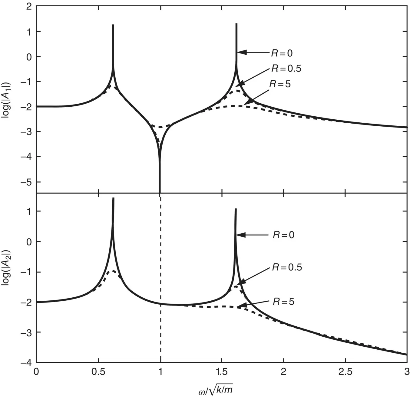
Figure 2.14 Forced response spectra of a damped two‐degree of freedom system.

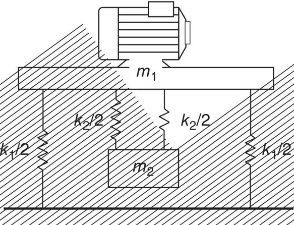
Figure 2.15 Undamped dynamic vibration absorber defined in Example 2.9.

All structural systems such as beams, columns, and plates are continuous systems with an infinite number of degrees of freedom. Consequently, a continuous system has an infinite number of natural frequencies and corresponding mode shapes. Although easier, modeling a structure using a finite number of degrees of freedom provides just an approximation of the behavior of the system. The analysis of continuous systems requires the solution of partial differential equations. However, analytical solutions to partial differential equations are often difficult to obtain and numerical or approximate methods are usually employed to analyze continuous systems in particular at high frequencies. However, flexural vibration of some common structural elements can be analytically studied. Sound radiation can be produced by the vibration of these structural elements. Such is the case of the vibration of thin beams, thin plates and thin cylindrical shells that will be discussed in the following sections.

If we ignore the effects of axial loads, rotary inertia, and shear deformation, the equation governing the free transverse vibrations w ( x , t ) of a uniform beam is given by the Euler–Bernoulli beam theory as [10, 13]

(2.51)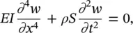

where E is the Young's modulus, ρ is the mass density, I is the cross‐sectional moment of inertia, and S is the cross‐sectional area. Assuming harmonic vibrations in the form

(2.52)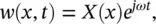

and substituting w ( x , t ) from Eq. (2.52)into Eq. (2.51)we get

(2.53)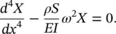

The solution of Eq. (2.53)is

(2.54)

where λ = ( ω 2 ρS / EI ) 1/4and the C 's are arbitrary constants that depend upon the boundary conditions (the deflections, slope, bending moment, and shear force constraints). Classical boundary conditions for a beam are

(2.55)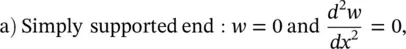

(2.56)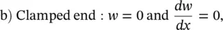

(2.57)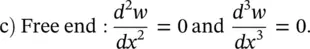

A very important practical case is a cantilever beam (clamped‐free beam) of length L . In this case, the deflection and slope are zero at the clamped end, while the bending moment and shear force are zero at the free end, i.e.

(2.58)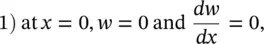

(2.59)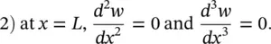

Substituting the boundary conditions Eq. (2.58)and Eq. (2.59)into Eq. (2.54), we find that C 2= − C 4, and we obtain the equation

(2.60)

The roots of the transcendental Eq. (2.60)can be obtained numerically. The first four roots are λ 1 L = 1.875, λ 2 L = 4.694, λ 3 L = 7.855, and λ 4 L = 10.996. For large values of n , the roots can be calculated using the equation

(2.61)

Noting that , we can solve for ω nso that the first four natural frequencies of the cantilever beam are