Malcolm J. Crocker - Engineering Acoustics

The simple mass‐spring‐damper system excited by a harmonic force was discussed in the preceding sections assuming a single mass which could move in one axis only. This single‐degree‐of‐freedom system idealization is reasonable when the mass is fairly rigid, the springs are lightweight and its motion can be described by means of one variable. For simple systems vibrating at low frequencies, it is also often possible to represent continuous systems with discrete or lumped parameter models. However, real systems have more than just one degree of freedom and, consequently, more than one natural frequency of vibration. For example, systems with more than one mass or systems in which a mass has considerable translation or rotation in more than one direction need to be modeled as multi‐degree of freedom systems. In multi‐degree of freedom systems, we have to consider the relationship between the motions of the various masses, i.e. their relative motion.

The general form of the equation that governs the forced vibration of an n ‐degree‐of‐freedom linear system with viscous damping can be written in matrix form as

(2.22)

where [ M ] is the n × n mass matrix, [ R ] is the n × n damping matrix (that incorporates viscous damping terms in the matrix formulation), [ K ] is the n × n stiffness matrix, qis the n ‐dimensional column vector of time‐dependent displacements, and f( t ) is the n ‐dimensional column vector of dynamic forces that act on the system. Therefore, the system governed by Eq. (2.22)exhibits motion which is governed by a set of n simultaneously second‐order differential equations. These equations can be derived using either Newton's laws for free body diagrams or energy methods. In particular, it can be shown that the mass and stiffness matrix are symmetric. This fact is assured if energy methods are used to derive the differential equations. However, symmetric mass and stiffness matrices can also be obtained after algebraic manipulation of the equations. In general, damping matrices are not symmetric unless the system is proportionally damped, i.e. the damping matrix is a linear combination of the mass matrix and stiffness matrix.

The algebraic complexity of the solution grows exponentially with the number of degrees of freedom and the general solution of Eq. (2.22)can be difficult to obtain for systems with a large number of degrees of freedom. Therefore, approximate and numerical approaches are often required to obtain the vibration properties and system response of a multi‐degree of freedom system.

By free vibration, we mean that the system is set into motion by some forces which then cease (at t = 0) and the system is then allowed to vibrate freely for t > 0 with no external forces applied. First we will consider a free undamped multi‐degree of freedom system, i.e. [ R ] = [0] and f( t ) = 0. Therefore, Eq. (2.22)now becomes

(2.23)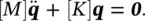

Similarly to the case of the single‐degree‐of‐freedom system discussed in Section 2.3, we assume harmonic solutions in the form

(2.24)

where Ais the vector of amplitudes. Substituting Eq. (2.24)into (2.23)yields

(2.25)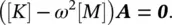

Equation (2.25)has a nontrivial solution if and only if the coefficient matrix ([ K ] − ω 2[ M ]) is singular, that is the determinant of this coefficient matrix is zero,

(2.26)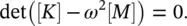

Equation (2.26)is called the characteristic equation (or characteristic polynomial) which leads to a polynomial of order n in ω 2. The roots of this polynomial, denoted as (for i = 1, 2, …, n ), are called the characteristic values (or eigenvalues). The square root of these numbers, ω iare called the natural frequencies of the undamped multi‐degree of freedom system and they can be arranged in increasing order of magnitude by ω 1≤ ω 2≤ … ≤ ω n. The lowest frequency ω 1is referred to as the fundamental frequency. The characteristic equation has only real roots due to the symmetry of the mass and stiffness matrices. In general, all the roots are distinct except in degenerate cases.

Note that are the eigenvalues of the matrix [ M ] −1[ K ], where [ M ] −1is the inverse of [ M ]. Associated with each characteristic value , there is an n ‐dimensional column linearly independent vector called the characteristic vector (or eigenvector) A iwhich is referred to as the i ‐th natural mode (normal mode, principal mode or mode shape) [10–13]. A iis obtained from the homogeneous system of equations represented by Eq. (2.27)as

(2.27)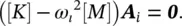

Since the system of equations represented by Eq. (2.27)is homogeneous, the mode shape is not unique. However, if is not a repeated root of the characteristic equation then there is only one linearly independent nontrivial solution of Eq. (2.27). The eigenvector is unique only to an arbitrary multiplicative constant [13]. It can be shown that the mode shapes are orthogonal. This property is important and allows a set of n decoupled differential equations of motion of a multi‐degree of freedom system to be obtained by using a modal transformation [10].

Solving Eq. (2.27)and replacing it into Eq. (2.24), we obtain a set of n linearly independent solutions q i= A iexp{ jω i t } of Eq. (2.23). Thus, the total solution can be expressed as a linear combination of them,

(2.28)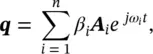

where β iare arbitrary constants which can be determined from initial conditions [usually with initial displacements and velocities q( t = 0) and ]. Equation (2.28)represents the superposition of all modes of vibration of the multi‐degree of freedom system.