Malcolm J. Crocker - Engineering Acoustics

Thus the static deflection d of the mass is

(2.8a)

The distance d is normally called the static deflection of the mass; we define a new displacement coordinate system, where Y = 0 is the location of the mass after the gravity force is allowed to compress the spring.

Suppose now we displace the mass a distance y from its equilibrium position and release it; then it will oscillate about this position. We will measure the deflection from the equilibrium position of the mass (see Figure 2.5b). Newton's law states that force is equal to mass × acceleration. Forces and deflections are again assumed positive upward, and thus

(2.9)

Let us assume a solution to Eq. (2.9)of the form y = A sin( ωt + φ ). Then upon substitution into Eq. (2.9)we obtain

We see our solution satisfies Eq. (2.9)only if

The system vibrates with free vibration at an angular frequency ω rad/s. This frequency, ω , which is generally known as the natural angular frequency, depends only on the stiffness K and mass M . We normally signify this so‐called natural frequency with the subscript n . And so

and from Eq. (3.2)

(2.10)

The frequency, f nhertz, is known as the natural frequency of the mass on the spring. This result, Eq. (2.10), looks physically correct since if K increases (with M constant), f nincreases. If M increases with K constant, f ndecreases. These are the results we also find in practice.

A machine of mass 600 kg is mounted on four springs of stiffness 2 × 10 5N/m each. Determine the natural frequency of the system

We model the system as a hanging spring‐mass system (see Figure 2.5). Equation (2.9)governs the displacement of the machine from its static‐equilibrium position. Since we have four equal springs, the equivalent stiffness is 4 × 2 × 10 5= 8 × 10 5N/m. The natural frequency is then determined using Eq. (2.10)as

We have seen that a solution to Eq. (2.9)is y = A sin( ωt + ϕ ) or the same as Eq. (2.3). Hence we know that any system that has a restoring force that is proportional to the displacement will have a displacement that is simple harmonic . This is an alternative definition to that given in Section 2.2for simple harmonic motion .

b) Free Vibration – Damped

Many mechanical systems can be adequately described by the simple mass–spring system just discussed above. However, for some purposes it is necessary to include the effects of losses (sometimes called damping). This is normally done by including a viscous damper in the system (see Figure 2.6). See Refs. [8, 9] for further discussion on passive damping. With viscous or “coulomb” damping the friction or damping force F dis assumed to be proportional to the velocity, dy/dt . If the constant of proportionality is R , then the damping force F don the mass is

(2.11)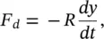

and Eq. (2.9)becomes

(2.12)

or equivalently

(2.13)

where the dots represent single and double differentiation with respect to time.

Figure 2.6 Movement of damped simple system.

The solution of Eq. (2.13)is most conveniently found by assuming a solution of the form: y is the real part of A e jλtwhere Ais a complex number and λ is an arbitrary constant to be determined. By substituting y = A e jλtinto Eq. (2.13)and assuming that the damping constant R is small, R < (4 MK) 1/2(which is true in most engineering applications), the solution is found that:

(2.14)

Here ω dis known as the damped “natural” angular frequency:

(2.15)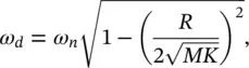

where ω nis the undamped natural frequency . The motion described by Eq. (2.14)is plotted in Figure 2.7.

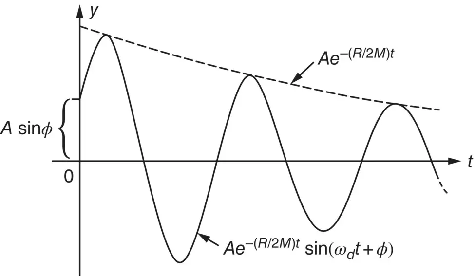
Figure 2.7 Motion of a damped mass–spring system, R < (4 MK ) 1/2.

The amplitude of the motion decreases with time unlike that for undamped motion (see Figure 2.3). If the damping is increased until R equals (4 MK ) 1/2, the damping is then called critical, R crit= (4 MK ) 1/2. In this case, if the mass in Figure 2.6is displaced, it gradually returns to its equilibrium position and the displacement never becomes negative. In other words, there is no oscillation or vibration. If R > (4 MK ) 1/2, the system is said to be overdamped.

The ratio of the damping constant R to the critical damping constant R critis called the damping ratio δ :

(2.16)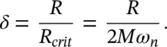

In most engineering cases, the damping ratio, δ , in a structure is hard to predict and is of the order of 0.01–0.1. There are, however, several ways to measure damping experimentally [8, 9].