Malcolm J. Crocker - Engineering Acoustics

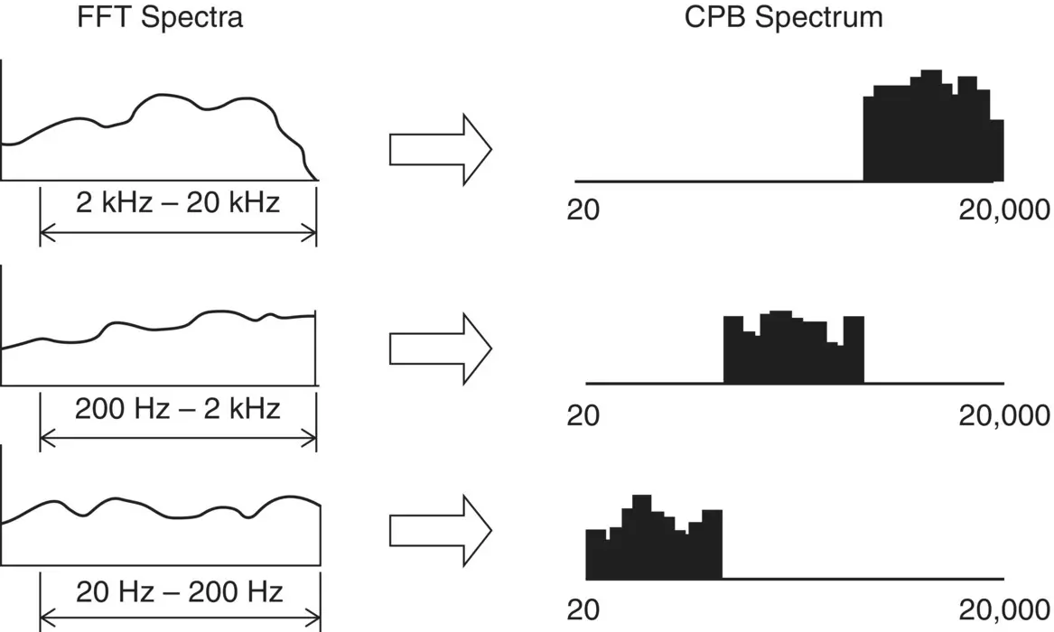
Figure 1.13 Conversion from FFT spectra to a constant percentage bandwidth (CPB) spectrum [21].

With the development of and decreasing prices of computer technologies, traditional FFT‐based instruments are becoming replaced by computer‐based instruments because of the processing, interfacing, and networking power of computers. Thus, digital signal processors can be replaced by specific software running on a personal computer. Computation speed reduction is not a problem because normally, calculations are made faster than they can be displayed. For data acquisition, since computers have hard drives of huge data storage capabilities, computers have advantages over traditional data logging equipment [20]. In addition, users can now develop their own programs to design instruments for noise and vibration signal analysis.

1 1 Piersol, A.G. and Bendat, J.S. (2010). Random Data: Analysis and Measurement Procedures, 4e. Hoboken, NJ: Wiley.

2 2 Piersol, A.G. and Bendat, J.S. (1993). Engineering Applications of Correlation and Spectral Analysis, 2e. New York: Wiley.

3 3 Oppenheim, A.V., Willsky, A.S., and Hamid, S. (1997). Signals and Systems, 2e. Harlow: Pearson.

4 4 Bracewell, R.N. (1999). The Fourier Transform and Its Applications, 3e. New York: McGraw‐Hill.

5 5 Tohyama, M. and Koike, T. (1998). Fundamentals of Acoustic Signal Processing. London: Academic Press.

6 6 Hansen, E.W. (2014). Fourier Transforms: Principles and Applications. New York: Wiley.

7 7 Newland, D.E. (2005). An Introduction to Random Vibrations, Spectral & Wavelet Analysis, 3e. Mineola, NY: Dover.

8 8 Lathi, B.P. and Ding, Z. (2009). Modern Digital and Analog Communication Systems, 4e. Oxford: Oxford University Press.

9 9 Magrab, E.B. and Blomquist, D.S. (1971). Measurement of Time‐Varying Phenomena: Fundamentals and Applications. New York: Interscience.

10 10 Herlufsen, H., Gade, S., and Zaveri, H.K. (2007). Analyzers and signal generators. In: Handbook of Noise and Vibration Control (ed. M.J. Crocker), 470–485. New York: Wiley.

11 11 Fourier, J. (1822). Théorie analytique de la chaleur. Paris: Firmin Didot Père et Fils.

12 12 Randall, R.B. (1987). Frequency Analysis, 3e. Naerum, Denmark: Bruel & Kjaer.

13 13 Piersol, A.G. (2007). Signal Analysis. In: Handbook of Noise and Vibration Control (ed. M.J. Crocker), 493–500. New York: Wiley.

14 14 Oppenheim, A.V. and Schafer, R.W. (2009). Discrete‐Time Signal Processing, 3e. Upper Saddle River, NJ: Prentice‐Hall.

15 15 ISO R 266:1997 (1997) Acoustics – Preferred Frequencies. Geneva: International Standards Organization.

16 16 IEC 1260:1995‐07 (1995) Electroacoustics – Octave‐band and Fractional‐octave‐band Filters, Class 1. Geneva: International Electrotechnical Commission.

17 17 ANSI S1.11‐2004 (2004) Specification for Octave‐band and Fractional‐octave‐band Analog and Digital Filters, Class 1. New York: American National Standards Institute.

18 18 Cooley, J.W. and Tukey, J.W. (1965). An algorithm for the machine computation of the complex Fourier series. Math. Comput. 19 (90): 297–301.

19 19 Duhamel, P. and Vetterli, M. (1990). Fast Fourier Transforms: a tutorial review and a state of the art. Signal Process. 19: 259–299.

20 20 Li, Z. and Crocker, M.J. (2007). Equipment for data acquisition. In: Handbook of Noise and Vibration Control (ed. M.J. Crocker), 486–492. New York: Wiley.

21 21 Randall, R.B. (2007). Noise and vibration data analysis. In: Handbook of Noise and Vibration Control (ed. M.J. Crocker), 549–564. New York: Wiley.

The vibrations in machines and structures result in oscillatory motion that propagates in air and/or water and that is known as sound. The simplest type of oscillation in vibration and sound phenomena is known as simple harmonic motion, which can be shown to be sinusoidal in time. Simple harmonic motion is of academic interest because it is easy to treat and manipulate mathematically; but it is also of practical interest. Most musical instruments make tones that are approximately periodic and simple harmonic in nature. Some machines (such as electric motors, fans, gears, etc.) vibrate and make sounds that have pure tone components. Musical instruments and machines normally produce several pure tones simultaneously. The simplest vibration to analyze is that of a mass–spring–damper system. This elementary system is a useful model for the study of many simple vibration problems. In this chapter we will discuss some simple theory that is useful in the control of noise and vibration. For more extensive discussions on sound and vibration fundamentals, the reader is referred to more detailed treatments available in several books [1–7]. We start off by discussing simple harmonic motion. This is because very often oscillatory motion, whether it be the vibration of a body or the propagation of a sound wave, is like this idealized case. Next, we introduce the ideas of period, frequency, phase, displacement, velocity, and acceleration. Then we study free and forced vibration of a simple mass–spring system and the influence of damping forces on the system. In Section 2.4we discuss the vibration of systems of several degrees of freedom and Section 2.5describes the vibration of continuous systems. This chapter also serves as an introduction to some of the topics that follow in this book.

The motion of vibrating systems such as parts of machines, and the variation of sound pressure with time is often said to be simple harmonic. Let us examine what is meant by simple harmonic motion.

Suppose a point P is revolving around an origin O with a constant angular velocity ω , as shown in Figure 2.1.

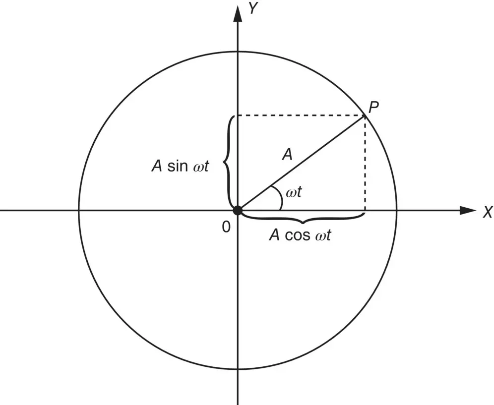
Figure 2.1 Representation of simple harmonic motion by projection of the rotating vector A on the X ‐ or Y ‐axis.

If the vector OP is aligned in the direction OX when time t = 0, then after t seconds the angle between OP and OX is ωt . Suppose OP has a length A , then the projection on the X‐ axis is A cos( ωt ) and on the Y‐ axis, A sin( ωt ). The variation of the projected length on either the X‐ axis or the Y‐ axis with time is said to represent simple harmonic motion.

It is easy to generate a displacement vs. time plot with this model, as is shown in Figure 2.2. The projections on the X‐ axis and Y‐ axis are as before. If we move the circle to the right at a constant speed, then the point P traces out a curve y = A sin( ωt ), horizontally. If we move the circle vertically upwards at the same speed, then the point P would trace out a curve x = A cos( ωt ), vertically.

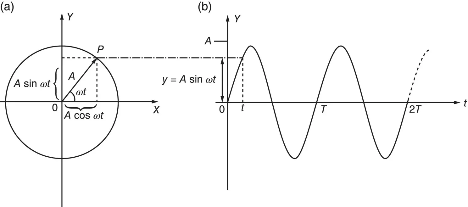
Figure 2.2 Simple harmonic motion.

The motion is seen to repeat itself every time the vector OP rotates once (in Figure 2.1) or after time T seconds (in Figures 2.2and 2.3). When the motion has repeated itself, the displacement y is said to have gone through one cycle . The number of cycles that occur per second is called the frequency f . Frequency may be expressed in cycles per second or, equivalently in hertz, or as abbreviated, Hz. The use of hertz or Hz is preferable because this has become internationally agreed upon as the unit of frequency. (Note cycles per second = hertz.) Thus