Malcolm J. Crocker - Engineering Acoustics

It is illustrative to consider an example of a two‐degree‐of‐freedom system, as the one shown in Figure 2.11, because its analysis can easily be extrapolated to systems with many degrees of freedom.

The two‐coordinates x 1and x 2uniquely define the position of the system illustrated in Figure 2.11if it is constrained to move in the x ‐direction. The equations of motion of the system are:

(2.29a)

and

(2.29b)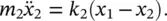

We observe that the equations of motion are coupled, that is to say the motion x 1is influenced by the motion x 2and vice versa. Equation (2.29)can be written in matrix form as

(2.30)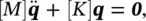

where q= , 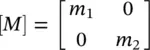and .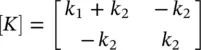

Equation (2.26)gives the characteristic equation

(2.31)

For simplicity, consider the situation where m 1= m 2= m and k 1= k 2= k . Then, Eq. (2.31)becomes

(2.32)

Solving Eq. (2.32)gives the natural frequencies of the system as

(2.33)

Note that Eq. (2.32)has four roots, the additional two being − ω 1and − ω 2. However, since these negative frequencies have no physical meaning, they can be ignored. For each positive natural frequency there is an associated eigenvector that is obtained from Eq. (2.27). Substitution of Eq. (2.33)into Eq. (2.27)and solving for A i, yields:

(2.34a)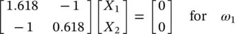

and

(2.34b)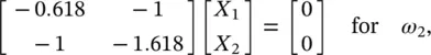

where X 1and X 2are the elements of vector A i. Equations (2.34a)and (2.34b)are homogenous, so that no unique solution is possible. Indeed, a solution with all its components multiplied by the same constant is also a solution [11]. Choosing arbitrarily X 1= 1 and solving Eq. (2.34)we get the eigenvectors

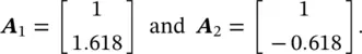
When used to describe the motion of a multi‐degree of freedom system, the mode shape refers to the amplitude ratio. These ratios are possible to obtain because their absolute values are arbitrary [12]. Thus, we express the mode shapes as the ratio of the amplitudes X 1/ X 2. Then, for ω 1, X 1/ X 2= 0.618 and for ω 2, X 1/ X 2= −1.618. These ratios can be represented in the mode plot of Figure 2.12. We note that when this simple two‐degree of freedom system vibrates at the first (fundamental) natural frequency ω 1, the two masses vibrate in phase ( Figure 2.12a). When the system vibrates at the second natural frequency ω 2, the two masses vibrate out of phase ( Figure 2.12b).

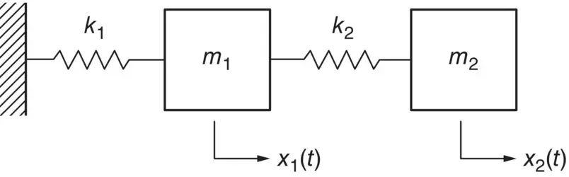
Figure 2.11 Two‐degree‐of‐freedom system.

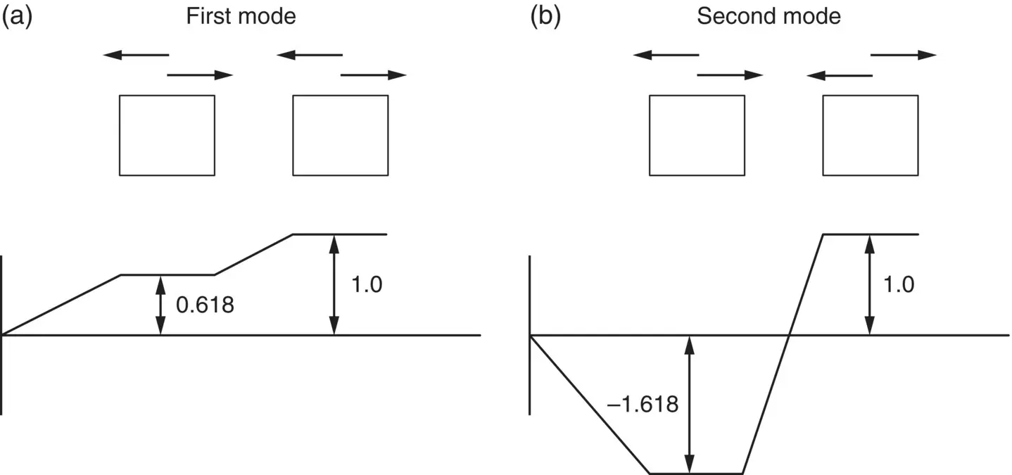
Figure 2.12 Mode shapes for the two‐degree of freedom system shown in Figure 2.11; (a) first mode, (b) second mode.

By forced vibration, we mean that the system is vibrating under the influence of continuous (external) forces that do not cease. The total response of a multi‐degree of freedom system due to a force excitation is the sum of a homogeneous solution and a particular solution. The homogenous solution depends upon the system properties while the particular solution is the response due to the particular form of excitation. The homogenous solution is often ignored for a system subjected to a periodic vibration for being of lesser practical importance than the particular solution. For a general form of excitation, a closed‐form solution of a multi‐degree of freedom system can be very difficult to obtain and numerical methods are often used.

The equations of motion of an n ‐degree‐of‐freedom undamped linear system excited by simple harmonic forces at some arbitrary angular forcing frequency ω (all excitation terms at the same phase) can be expressed in matrix form as

(2.35)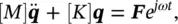

where Fis an n ‐dimensional complex column vector of dynamic amplitude forces. We assume harmonic solutions of the form

(2.36)

where Ais a vector of undetermined amplitudes. Substituting Eq. (2.36)into (2.35)leads to

(2.37)

A unique solution of Eq. (2.37)exists unless

(2.38)

which has the same form as Eq. (2.26). Equation (2.38)is satisfied only when the forcing frequency coincides with one of the system's natural frequencies. In this condition, called resonance, the response of the system grows linearly with time and thus use of the solution Eq. (2.36)is unsuitable. When a solution of Eq. (2.37)exists, the amplitudes can be determined as [13]