Spectroscopy for Materials Characterization

(1.94)

giving the amplitude of absorption for the transition from the ground vibrational level of the electronic ground state to the m th vibrational level of the excited electronic state, where E 00is the zero‐phonon line energy. Analogously, for the emission process, one can write

(1.95)

considering that at room temperature, after the absorption process, the system relaxes to the lowest vibrational level in the excited state, as shown by the dash‐dotted arrow in Figure 1.5, and then it goes back to the electronic ground state, occupying one of the many vibrational levels depending on the | M n0| 2factor. On the basis of the wavefunctions of the harmonic oscillator, it can be demonstrated that [5, 15, 18, 19]

(1.96)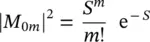

where the Huang–Rhys factor S has been inserted [19]

(1.97)

connecting the Stokes shift of the absorption and emission transitions to the vibrational energy of the oscillator considered. Equation (1.96)is a Poisson distribution with variance S , standard deviation , and average value S [20]. The Huang–Rhys factor measures the nuclear relaxation energy Δ U in units of the vibrational quantum of energy ℏω . In particular, the larger relaxation occurs in the presence of a strong electron–phonon coupling, implying that when the electron is excited, a large modification of the equilibrium position of nuclei occurs, with the ensuing relative shifts of the parabola describing the energy of the ground and of the excited state, as schematized in Figure 1.5[15, 18]. It is interesting to observe that on increasing the Huang–Rhys factor, the lineshape of the considered transition, given by the distribution of | M 0m| 2, changes from strongly asymmetric (0 < S < 1) with predominance of the zero‐phonon line, to gently asymmetric (1 < S < 6) with residual of the ZPL, to symmetric and almost Gaussian ( S > 10) with small contribution of the ZPL [15]. The Huang–Rhys factor can be determined from the Stokes shift once the vibration frequency is known using (1.87)and (1.97). Furthermore, S can be determined from the area of the ZPL and the total area of the absorption (or emission) bands. In fact, starting from (1.96), it can be shown that

(1.98)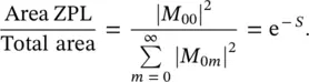

Finally, for large values of S, the variance of the Poisson distribution is equal to S and the spectral variance in terms of ℏω will be S ( ℏω ) 2. From the Gaussian profile reported by (1.78), it is then determined that

(1.99)

and the Huang–Rhys factor could be experimentally estimated. To conclude these considerations on the homogeneous lineshape, a more detailed treatment should include the many possible vibration degrees of freedom of a polyatomic molecule and replicas of the considered features have to be inserted with different Huang–Rhys factors for each mode [8, 18, 21].

In the previous paragraph, the simplest molecular model using the Born–Oppenheimer approximation enabled to determine the dipole moment matrix element (1.92). The first factor is related to the electronic wavefunction and the second factor is due to the nuclear wavefunction. It is usual to consider two contributions in the electronic wavefunction, the first due to the orbital motion and the second due to the spin degrees of freedom. The dipole moment matrix element can then be written

(1.100)

where the first factor accounts for the spatial dependence of the electron motion (orbital contribution), the second factor for the spin contribution, and the third factor for the nuclear vibration (Franck–Condon factor). Each of these factors contributes to the evaluation of the dipole moment matrix element, and they give rise to the selection rules for the vibronic transition [5, 8]. A given transition is usually called spin forbidden if

(1.101)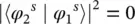

this is typically the most limiting rule. The dipole moment matrix element is related to the oscillator strength by Eq. (1.57)and to the experimental absorption through (1.56)and the molar extinction coefficient through (1.8); so, it is observed that the latter parameter is in the range (10 −5< ε < 10 0) M −1cm −1for spin forbidden transitions. When the orbital factor is null

(1.102)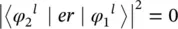

the transition is called orbitally forbidden and the range (10 0< ε < 10 3) M −1cm −1is found for the molar extinction coefficient. Finally, values (10 3< ε < 10 5) M −1cm −1typically pertain to allowed transitions. It is worth observing that these rules could not be strictly respected since in some cases the vibronic states could have a not pure spin or orbital angular momentum contribution, being instead a mixture of states [5, 8, 9].

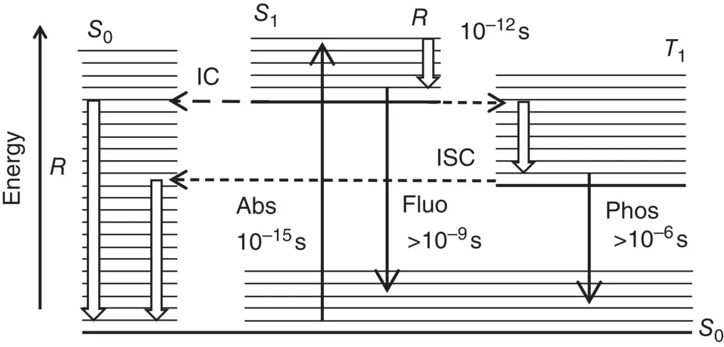
Figure 1.6Jablonski diagram for the transition processes of electrons among vibronic states. The electronic levels are labeled by S 0, S 1, T 1and thick horizontal lines, thinner horizontal lines mark the vibrational levels. Continuous arrows represent photon‐related (radiative) transitions; white arrows mark relaxation transitions among vibrational levels; short‐dashed arrows represent the intersystem crossing process (ISC); dashed line the internal conversion process. Typical times of the processes of absorption (Abs) fluorescence (Fluo), phosphorescence (Phos), and vibrational relaxation ( R ) are inserted.

The overall sequence of transitions occurring among the energy states of a molecule can now be described in more detail. Figure 1.6shows a schematic representation of the processes connecting the ground state S 0and the excited state S 1, assumed to be spin singlet states, and the excited spin triplet state T 1.