Sheila Annie Peters - Physiologically Based Pharmacokinetic (PBPK) Modeling and Simulations

Common routes of drug administration include per oral (PO), intramuscular (IM), subcutaneous (SC) intravenous (IV) bolus and infusion, and intrathecal (around the spinal cord). Other less common routes include buccal, sublingual, rectal, transdermal, inhalational, and topical. The oral route is the most preferred route, but it is not suitable for drugs that are not stable in the gut, like for example peptide and protein drugs.

Intravenous (IV) administration ensures rapid, complete drug availability for drugs that are not in the form of suspensions or oils, by bypassing absorption barriers. Drugs having poor oral bioavailability or causing unacceptable pain when administered intramuscularly or subcutaneously may be administered by this route. However, it is potentially hazardous, as the initial high drug concentration may elicit toxic effects. Therefore, the use of IV route is restricted to situations demanding a rapid onset of action as in anesthesia, emergency medicine etc. or, when the patient is persistently vomiting, is unconscious or is too young to safely swallow solid forms of medication. Controlled drug administration through IV infusions offers one way to mitigate the risk of toxicity, as the infusion may be halted in the unexpected event of adverse effects during administration. Apart from causing severe pain, intra‐arterial administration is associated with the risk of dangerous pressure buildup in the muscles leading to decreased blood flow and consequently to nerve and muscle damage. Intra‐arterial injections are therefore reserved to situations in which localizations to specific tissues are desired.

Drug elimination from the body may follow zero or first‐order kinetics ( Figure 1.1). In zero‐order kinetics, a constant amount of the drug is eliminated in a certain time (e.g., 20 mg per hour). In first‐order processes, a constant proportion of the drug is eliminated in a certain time (e.g., 20% per hour). Though relatively rare, zero‐order kinetics may be encountered in intravenous infusions as well as in elimination of some drugs (e.g. ethanol) but will not be further elaborated here.

The temporal changes in the drug concentrations following an IV bolus injection of 50 mg of a drug with first‐order kinetics are depicted in Figure 1.2. The slope and area under the curve ( AUC ) are the two parameters that can be extracted from the concentration‐time profile as shown in the semilogarithmic and linear plots respectively. Other useful pharmacokinetic parameters may be derived from these two parameters, as will become evident from the mathematical derivations below.

The first‐order rate equation depicting the rate of change of drug concentrations in the blood ( C ) is given by

(1.1)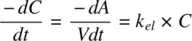

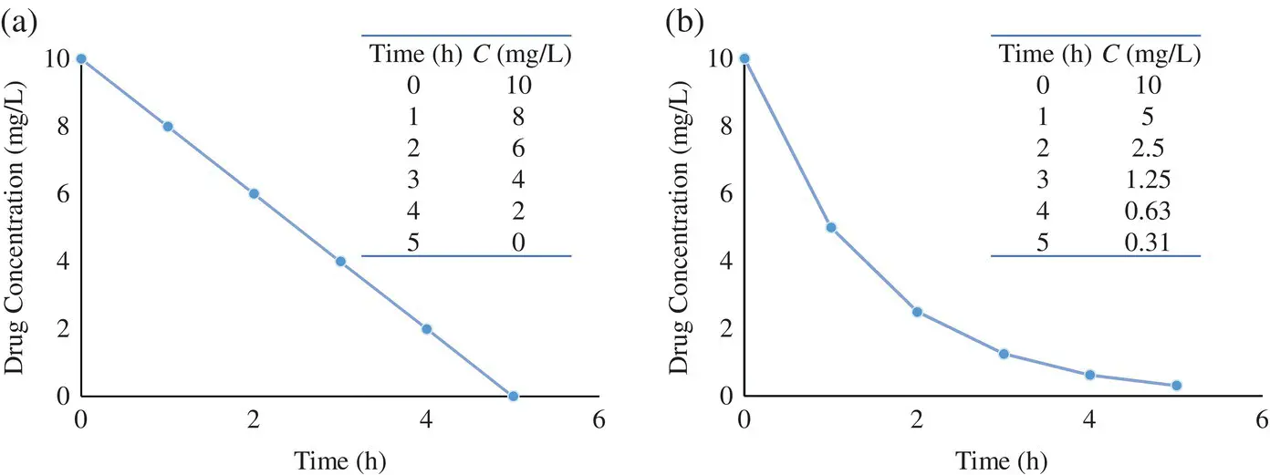
Figure 1.1. Temporal changes in drug concentrations for (a) zero‐order and (b) first‐order kinetics.

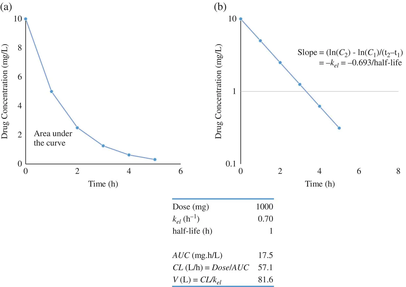
Figure 1.2. Linear (a) and semilogarithmic (b) plots of drug concentrations vs. time. Area under the curve (AUC) and slope are the two parameters that can be obtained from the plot. C 2and C 1are drug concentrations at times t 2and t 1respectively. k el, first‐order elimination rate constant; CL , is the total drug clearance; and V , volume of distribution.

(1.2)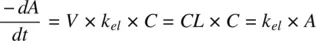

where A is the amount of drug in the body at any time, t , k elis the first‐order elimination rate constant, and V is the volume of distribution of the drug. The product of k eland V is defined as the total clearance, CL , of the drug from blood.

Integrating Equation 1.1( −dC/dt = k el× C ),

(1.3)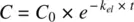

Taking natural logarithms on both sides,

(1.4)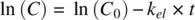

Thus, k elmay be obtained by measuring the slope of a semilogarithmic plot of drug concentration vs time ( Figure 1.2).

Similarly, integrating Equation 1.2( −dA/dt = k el× A ) yields

(1.5)

where A 0is the initial amount of drug in the body, the dose administered as IV bolus. Bringing A 0to the left‐hand side, Equation 1.5becomes,

(1.6)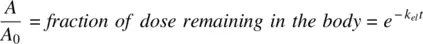

Taking the natural logarithms on both sides of the resulting equation leads to the following:

(1.7)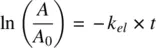

The half‐life ( t 1/2) of a drug, defined as the time taken for half of the administered drug to get eliminated from the body (time taken for drug amount in body to go from A 0, to A 0/2, or time taken for the drug concentration to be halved), is given by:

(1.8)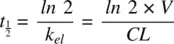

Using Equation 1.8, the half‐life of a drug can be calculated from the elimination rate constant k elwhich is obtained from the semilogarithmic plot of concentration vs. time ( Figure 1.2).

Integrating the Equation 1.2( −dA = CL × C dt ) yields

(1.9)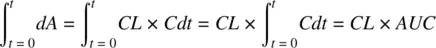

where AUC is the area under the drug concentration‐time profile ( Figure 1.2), which may be estimated from the plot by applying the trapezoidal rule. Recognizing that the integral dA over time 0 to t is the dose, Equation 1.9becomes,

(1.10)