Scott D. Sudhoff - Power Magnetic Devices
Здесь есть возможность читать онлайн «Scott D. Sudhoff - Power Magnetic Devices» — ознакомительный отрывок электронной книги совершенно бесплатно, а после прочтения отрывка купить полную версию. В некоторых случаях можно слушать аудио, скачать через торрент в формате fb2 и присутствует краткое содержание. Жанр: unrecognised, на английском языке. Описание произведения, (предисловие) а так же отзывы посетителей доступны на портале библиотеки ЛибКат.
- Название:Power Magnetic Devices
- Автор:
- Жанр:
- Год:неизвестен
- ISBN:нет данных
- Рейтинг книги:4 / 5. Голосов: 1
-
Избранное:Добавить в избранное
- Отзывы:
-
Ваша оценка:
Power Magnetic Devices: краткое содержание, описание и аннотация
Предлагаем к чтению аннотацию, описание, краткое содержание или предисловие (зависит от того, что написал сам автор книги «Power Magnetic Devices»). Если вы не нашли необходимую информацию о книге — напишите в комментариях, мы постараемся отыскать её.
Discover a cutting-edge discussion of the design process for power magnetic devices Power Magnetic Devices: A Multi-Objective Design Approach
Power Magnetic Devices
Power Magnetic Devices — читать онлайн ознакомительный отрывок
Ниже представлен текст книги, разбитый по страницам. Система сохранения места последней прочитанной страницы, позволяет с удобством читать онлайн бесплатно книгу «Power Magnetic Devices», без необходимости каждый раз заново искать на чём Вы остановились. Поставьте закладку, и сможете в любой момент перейти на страницу, на которой закончили чтение.
Интервал:
Закладка:
Let us consider the crossover, segregation, and mutation processes on a numerical example. Figure 1.9illustrates these operators. Therein g 1− g 4denote genes 1–genes 4 and c 1and c 2denote chromosomes 1 and 2, respectively. We start at the left of the diagram with the two parents θ p1and θ p2. The first operator applied is crossover. Assuming the crossover point is between the first and second bits in the first chromosome, and that no crossover occurs in the second chromosome, we arrive at θ a1and θ a2. The portions of the genetic code which have been acted on by the crossover operator are shown in bold. Next, chromosome segregation occurs. In this case, by a random choice the first child inherits the first chromosome from θ a2and the second chromosome from θ a1. The second child inherits the remaining chromosomes. Next, let us assume that mutation acts to change the status of the first bit of gene 3 in θ b2. This yields θ c1and θ c2, where the affected bit is again indicated in boldface.
At this point, the main points of a canonical GA have been described. This canonical form is the type of algorithm first developed by Holland. The canonical GA can also be used to explain the effectiveness of GAs using schema theory. A schema is a pattern of bits; one reason GAs are so effective is that they can be shown to exhibit an implicit parallelism in which all schema that result in higher than average fitness tend to propagate. The interested reader is referred to textbooks on GAs such as those by Goldberg [4,5].
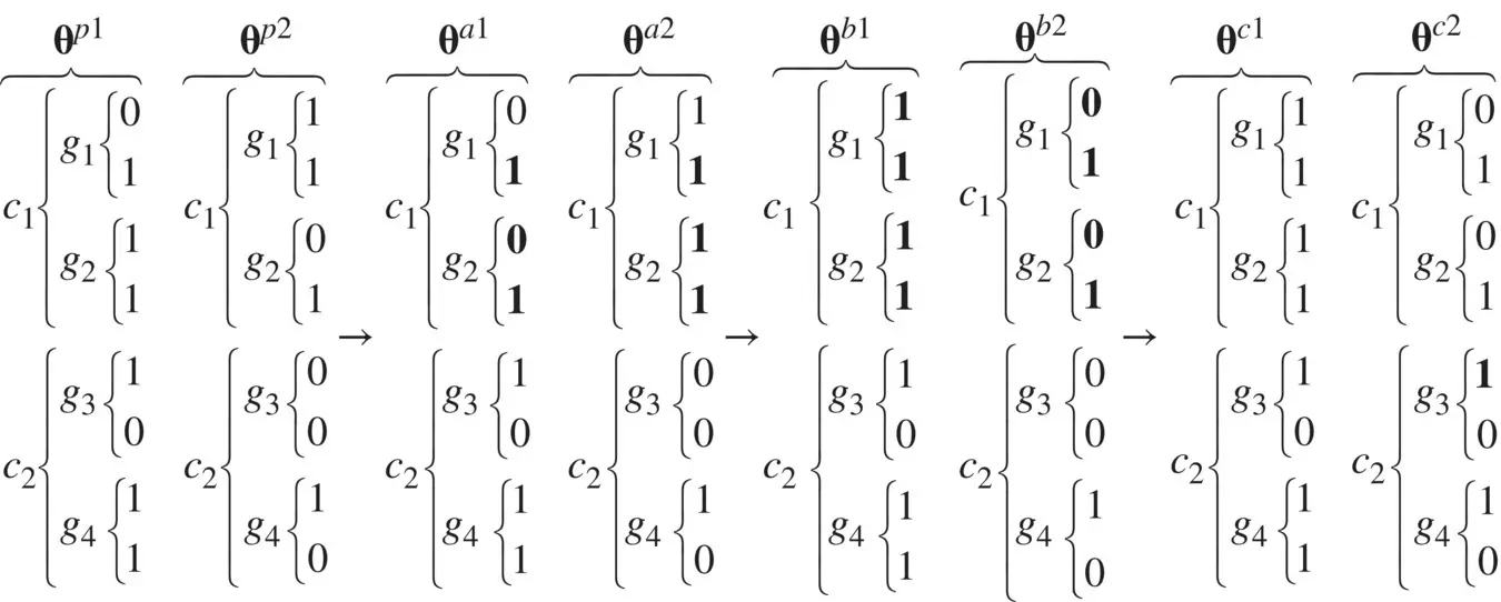
Figure 1.9 Chromosome crossover, segregation, and mutation in Example 1.5B.
At this point, an example would prove useful. Before embarking on such an example, however, it will prove useful to address one weakness of the GA. This weakness is the encoding algorithm. Although the representation of a member of the population as a string similar to that in DNA is intellectually appealing, it is also inconvenient. Further, a binary representation of real numbers suffers from finite resolution and the fact that sometimes large numbers of bits may need to change to accomplish a small change unless, for example, a Gray code scheme is used. As it turns out, it is possible to create a GA without encoding genes as strings and, instead, representing them with real numbers. Real‐coded GAs are simpler to write than their canonical counterparts and very effective. They will be our next topic.
1.6 Real‐Coded Genetic Algorithms
Real‐coded GAs are very similar to canonical GAs except that instead of each gene being represented as a binary string, each gene is represented by a real number. This proves convenient for coding purposes and makes representing each gene to the numerical precision of floating‐point numbers for a given machine (computer) straightforward. Beyond the change of the way in which a gene is represented, the algorithm presented in Figure 1.8is still applicable, though we will need to modify the encoding, crossover, and mutation operators.
Encoding
Let us begin our development by considering the form of the genetic code for the i th individual. In the case of the canonical GA, this was given by (1.5-2), where each element of θ iwas represented by a string. In the real‐coded GA, (1.5-2)still applies. However, instead of each element of θ ibeing represented by a string, in a real‐coded GA each element is represented by a real number. In fact, a real‐coded GA could be written such that θ i= x i. However, it will be convenient to provide a mapping of x ito θ iso that the gene values of θ ifall into the domain [0,1].
The mapping between x iand θ iis accomplished on a gene‐by‐gene basis. A simple choice is a linear map. Let x and θ denote a gene (element) of the x iand θ i. For a linear mapping, we have
(1.6-1) 
where j denotes the gene number and
(1.6-2) 
where x mn,jand x mx,jdenote the minimum and maximum values of the parameter.
Closely related to linear mapping is integer mapping, wherein x , x mn,j ,and x mx,jare integers. In this case, (1.6-2)still applies, but we require
(1.6-3) 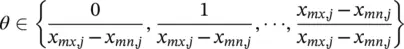
This mapping is useful in choosing, for example, between different types of steel in a design. If the third gene represented the type of steel used, and five types of steels were being considered, then x mn,3= 1, x mx,3= 5, and θ ∈ {0.00, 0.25, 0.50, 0.75, 1.00}.
In some cases, the domain of a parameter may span many decades in magnitude. If the domain of the parameter is always positive, then a logarithmic mapping is appropriate. In this case,
(1.6-4) 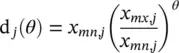
Crossover
In the case of the canonical GA, crossover is accomplished by breaking the subject chromosomes of the parents at the same point and interchanging them to form the corresponding chromosomes of the children. This interchange substantially alters the gene where the chromosome is interchanged, and it results in an interchange of genes falling after the interchange point.
There are several algorithms to achieve crossover in real‐coded GAs. One of them is single‐point crossover, which can be readily generalized to n ‐point crossover. This method is straightforward and is readily illustrated by the example shown in Figure 1.10. Therein, the genetic code for two parents, θ p1and θ p2, is shown. Observe that the elements of these vectors are real numbers in the domain [0,1]. In this algorithm, a crossover point is chosen at random and the genes after the crossover points are interchanged (these genes are in bold) to form two new genetic codes, θ a1and θ a2, which will become children after the application of additional genetic operators such as mutation.
Single‐point crossover is very similar to biological crossover. However, note that gene values cannot become altered using this operator. This limits the amount of genetic diversity that can be brought about.
Simple‐blend crossover can be used to increase the genetic diversity. Let us consider the j th gene of parents θ p1and θ p2. If the j th gene is being crossed over, the new gene values are determined by first computing a random number υ given by
(1.6-5) 
Интервал:
Закладка:
Похожие книги на «Power Magnetic Devices»
Представляем Вашему вниманию похожие книги на «Power Magnetic Devices» списком для выбора. Мы отобрали схожую по названию и смыслу литературу в надежде предоставить читателям больше вариантов отыскать новые, интересные, ещё непрочитанные произведения.


Обсуждение, отзывы о книге «Power Magnetic Devices» и просто собственные мнения читателей. Оставьте ваши комментарии, напишите, что Вы думаете о произведении, его смысле или главных героях. Укажите что конкретно понравилось, а что нет, и почему Вы так считаете.