Iam-Choon Khoo - Liquid Crystals

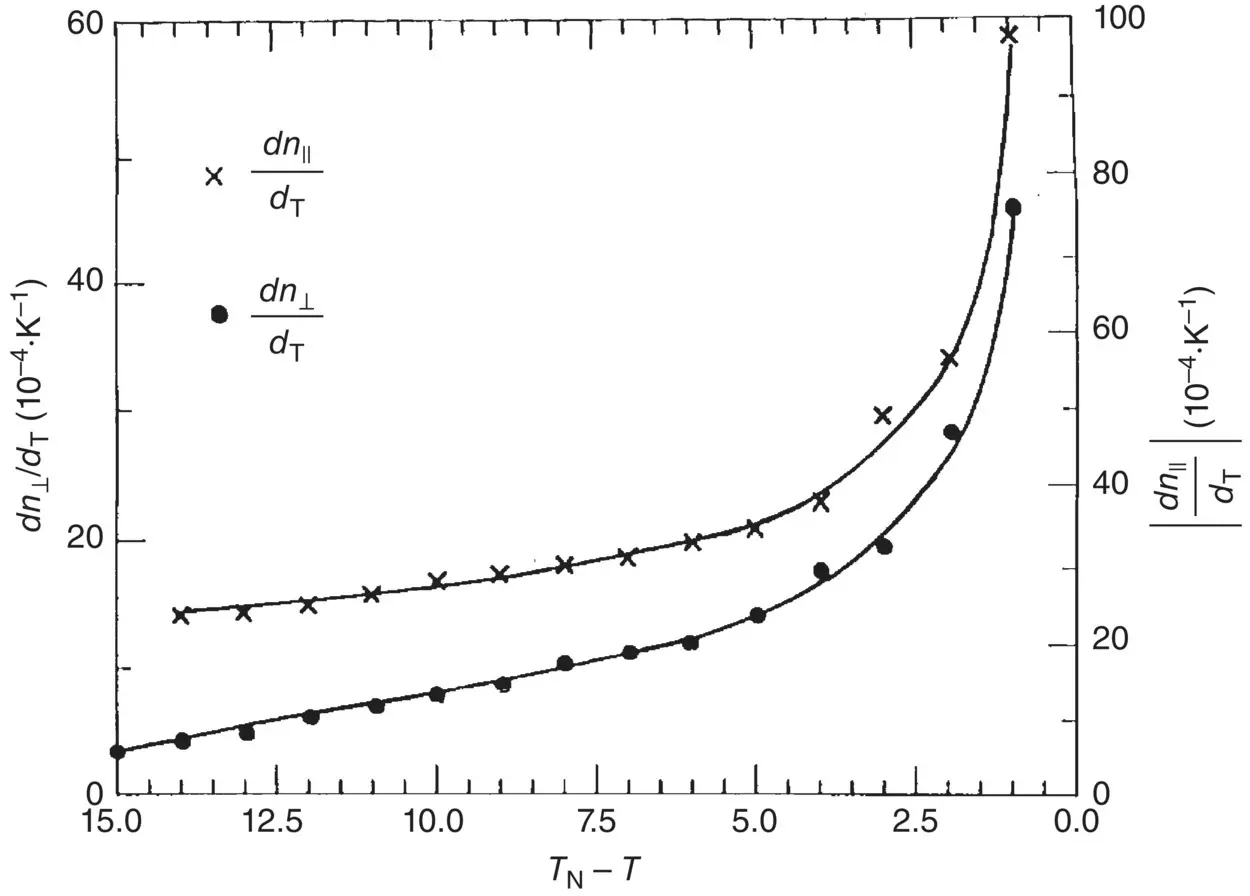
Figure 3.8. Plot of dn ||/ dT and dn ⊥/ dT for the liquid crystal for temperature near T c(after Khoo and Normandin [14] and Horn [15]). Solid curve is for visual aid only.

One of the most striking properties of liquid crystals is their ability to flow freely while exhibiting various anisotropic and crystalline properties. This dual nature of liquid crystals makes them very interesting materials to study; it also makes theoretical formalism very complex.

The main feature that distinguishes liquid crystals in their ordered mesophases (e.g. the nematic phase) from ordinary fluids is that their physical properties are dependent on the orientation of the director axis ; these orientation flow processes are necessarily coupled, except in very unusual cases (e.g. pure twisted deformation). Therefore, studies of the hydrodynamics of liquid crystals will involve a great deal more (anisotropic) parameters than studies of the hydrodynamics of ordinary liquids.

We begin our discussion by reviewing first the hydrodynamics of an ordinary fluid. This is followed by a discussion of the general hydrodynamics of liquid crystals. Specific cases involving a variety of flow‐orientational couplings are then treated.

Consider an elementary volume dV = dx dy dz of a fluid moving in space as shown in Figure 3.9. The following parameters are needed to describe its dynamics:

position vector: ,

velocity: ,

density: ,

pressure: , and

forces in general: .

In later chapters where we study laser‐induced acoustic (sound, density) waves in liquid crystals, or generally, when one deals with acoustic waves, it is necessary to assume that the density is a spatially and temporally varying function. In this chapter, however, we “decouple” such density wave excitation from all the processes under consideration and basically limit our attention to the flow and orientational effects of an incompressible fluid. In that case, we have

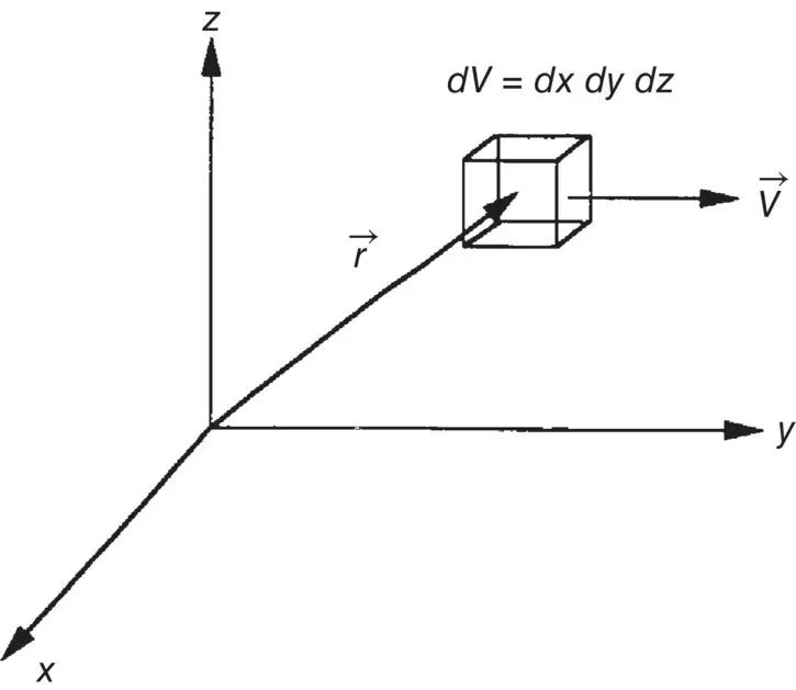
Figure 3.9. An elementary volume of fluid moving at velocity v ( r , t ) in space.

(3.50)

For all liquids, in fact for all gas particles or charges in motion, the equation of continuity also holds

(3.51)

This equation states that the total variation of over the surface of an enclosing volume is equal to the rate of decrease of the density. Since ∂ ρ /∂ t = 0, we thus have, from Eq. (3.51),

(3.52)

The equation of motion describing the acceleration of the fluid elements is simply Newton’s law:

(3.53a)

Studies of the hydrodynamics of liquids may be centered around this equation of motion, as we identify all the various origins and mechanisms of forces acting on the fluid elements and attempt to solve their motion in time and space.

We shall start with the left‐hand side of Eq. (3.53a). Since ,

(3.53b)

The force on the right‐hand side of Eq. (3.53a)comes from a variety of sources, including the pressure gradient −Δ ρ , viscous force , and external fields (electric, magnetic, optical, gravitational, etc.). Equation (3.53a)thus becomes

(3.54)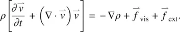

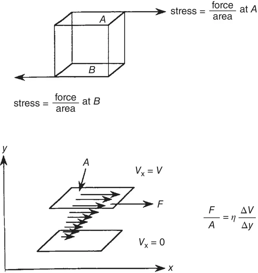
Figure 3.10. Stresses acting on opposite planes of an elementary volume of fluid.

Let us ignore the external field for the moment. The formulation of the equation of motion for a fluid element is complete once we identify the viscous forces. Note that, in analogy to the pressure gradient term, the viscous force is the space derivation of a quantity that has the unit of pressure (i.e. force per unit area). Such a quantity is termed the stress tensor σ (i.e. the force is caused by the gradient in the stress; see Figure 3.10). For example, the α component of may be expressed as

(3.55)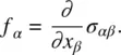

Accordingly, we may rewrite Eq. (3.54)as

(3.56)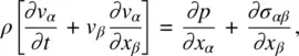

where summation over repeated indices is implicit.

By consideration of the fact that there is no force acting when the fluid velocity is a constant, the stress tensor is taken to be linear in the gradients of the velocity (see Figure 3.10), that is,

(3.57)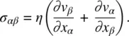

The proportionality constant η in Eq. (3.57)is the viscosity coefficient (in units of g cm −1S −1). Note that for fluid under uniform rotation (i.e. ), we have ∂ v β/∂ x α= −∂ v α/∂ x β, which means σ αβ= 0.