Manuel Pastor - Computational Geomechanics

or

(2.23b)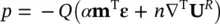

and thus we can eliminate p from (2.11) and (2.13).

The resulting system which is fully discussed in Zienkiewicz and Shiomi (1984) is not written down here as we shall derive this alternative form in Chapter 3using the total displacement of water U= U R+ uas the variable. It presents a very convenient basis for using a fully explicit temporal scheme of integration (see Chan et al. 1991) but it is not applicable for long‐term studies leading to steady‐state conditions, as the water displacement Uthen increases indefinitely.

It is fortunate that the inaccuracies of the u– p version are pronounced only in high‐frequency, short‐duration, phenomena, since, for such problems, we can conveniently use explicit temporal integration. Here a very small time increment can be used for the short time period considered (see Chapter 3).

Table 2.1summarizes various forms of governing equations used.

It is, of course, important to know the degree of approximation involved in various differential equation systems. Thus, it is of interest to know under what circumstances undrained conditions can be assumed, to define the behavior of the material and when the simplified equation system discussed in the previous section is applicable, without introducing serious error. An attempt to answer these problems was made by Zienkiewicz et al. (1980). The basis was the consideration of a one‐dimensional set of linearized equations of the full systems (2.11), (2.13), and (2.16) and of the approximations (2.20) and (2.21). The limiting case in which w i,i= 0 (representing undrained conditions) was also considered.

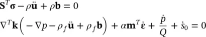
Table 2.1 Comparative sets of coupled equations governing deformation and flow.

u− w− p equations (exact) [(2.11), (2.13), and (2.16)]

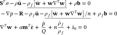u− p approximation for dynamics of lower frequencies. Exact for consolidation [(2.20), (2.21)]

u− U, only convective terms neglected (3.72)

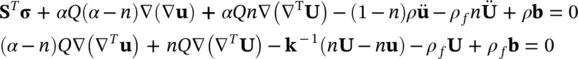In all the above

σ ″= σ+ α m p and d σ ″= D dε = DS d u

For all these conditions, the exact solution of the equation is possible. We consider thus that the only physical variation is in the vertical, x 1, direction ( x 1= x ) and then we have

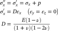
where D is called the one‐dimensional constrained modulus, E is Young’s modulus and ν is Poisson’s ratio of the linear elastic soil matrix, also

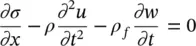
The differential equations are, in place of (2.11):

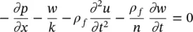
In place of (2.13):

and in place of (2.16):

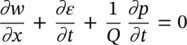
with

Taking K s→ ∞

For a periodic applied surface load

a periodic solution arises after the dissipation of the initial transient in the form

and a system of ordinary linear differential equations is obtained in the frequency domain which can be readily solved by standard procedure.

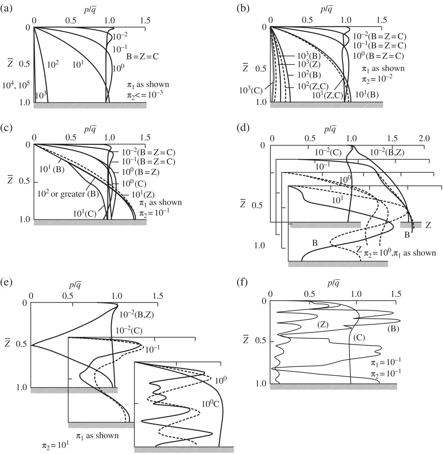
The boundary conditions imposed are as shown in Figure 2.1. Thus, at x = L , u = 0, w = 0, and at x = 0, σ x= q , p = 0.

In Figure 2.1(taken from Zienkiewicz et al. (1980)), we show a comparison of various numerical results obtained by various approximations:

1 exact solution (Biot’s, labelled B)

2 the u−p equation approximation (labelled Z)

3 the undrained assumption (w = 0) and

4 the consolidation equation obtained by omitting all acceleration terms (labelled C).

The reader will note that the results are plotted against two nondimensional coefficients:

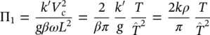
where k′ and k are the two definitions of permeability discussed earlier.

In the above

where L is a typical length such as the length of the one‐dimensional soil column under consideration, g is the gravitational acceleration,

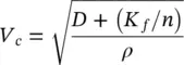
is the speed of sound, is the natural vibration period and T is the period of excitation.

The second nondimensional parameter is defined as