Manuel Pastor - Computational Geomechanics
Здесь есть возможность читать онлайн «Manuel Pastor - Computational Geomechanics» — ознакомительный отрывок электронной книги совершенно бесплатно, а после прочтения отрывка купить полную версию. В некоторых случаях можно слушать аудио, скачать через торрент в формате fb2 и присутствует краткое содержание. Жанр: unrecognised, на английском языке. Описание произведения, (предисловие) а так же отзывы посетителей доступны на портале библиотеки ЛибКат.

- Название:Computational Geomechanics
- Автор:
- Жанр:
- Год:неизвестен
- ISBN:нет данных
- Рейтинг книги:4 / 5. Голосов: 1
-
Избранное:Добавить в избранное
- Отзывы:
-
Ваша оценка:
Computational Geomechanics: краткое содержание, описание и аннотация
Предлагаем к чтению аннотацию, описание, краткое содержание или предисловие (зависит от того, что написал сам автор книги «Computational Geomechanics»). Если вы не нашли необходимую информацию о книге — напишите в комментариях, мы постараемся отыскать её.
Computational Geomechanics: Theory and Applications, Second Edition
Computational Geomechanics — читать онлайн ознакомительный отрывок
Ниже представлен текст книги, разбитый по страницам. Система сохранения места последней прочитанной страницы, позволяет с удобством читать онлайн бесплатно книгу «Computational Geomechanics», без необходимости каждый раз заново искать на чём Вы остановились. Поставьте закладку, и сможете в любой момент перейти на страницу, на которой закончили чтение.
Интервал:
Закладка:
Equations (2.11), (2.13), and (2.16) together with appropriate constitutive relations specified in the manner of (2.3) define the behavior of the solid together with its pore pressure in both static and dynamic conditions. The unknown variables in this system are:
The pressure of fluid (water), p ≡ pw
The velocities of fluid flow wi or w
The displacements of the solid matrix ui or u.
The boundary condition imposed on these variables will complete the problem. These boundary conditions are:
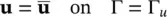
1 For the total momentum balance on the part of the boundary Γt, we specify the total traction ti(t) (or in terms of the total stress σij nj (σ⋅ G) with ni being the ith component of the normal at the boundary and G is the appropriate vectorial equivalence) while for Γu, the displacement ui(u), is given.
2 For the fluid phase, again the boundary is divided into two parts Γp on which the values of p are specified and Γw where the normal outflow wn is prescribed (for instance, a zero value for the normal outward velocity on an impermeable boundary).
Summarizing, for the overall assembly, we can thus write
(2.18) 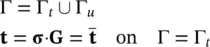
and
Further
(2.19a) 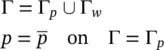
and
(2.19b) 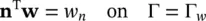
It is of interest to note, as shown by Zienkiewicz (1982), that some typical soil constants are implied in the formulation. For instance, we note from (2.16) that for undrained behavior , when w i,i= 0, i.e. with no net outflow, we have (neglecting the last two terms which are of the second order).
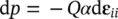
or
and
or
If the pressure change d p is considered as a fraction of the mean total stress change m Td σ /3 or d σ ii/3, we obtain the so‐called B soil parameter (Skempton 1954) as
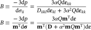
Using the assumption that the material is isotropic so that
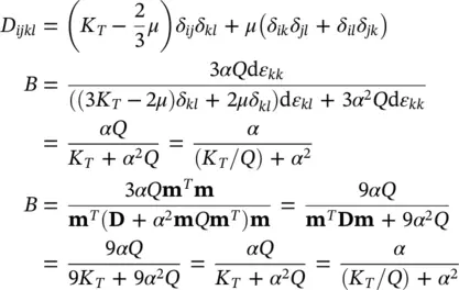
where K Tis (as defined in equation (1.10), the bulk modulus of the solid phase and μ is once again Lamé’s constant. B has, of course, a value approaching unity for soil but can be considerably lower for concrete or rock. Further, for unsaturated soils, the value will be much lower (Terzaghi 1925; Lambe and Whitman 1969; Craig 1992).
2.2.2 Simplified Equation Sets ( u – p Form)
The governing equation set (2.11), (2.13), and (2.16) together with the auxiliary definition system can, of course, be used directly in numerical solution as shown by Zienkiewicz and Shiomi (1984). This system is suitable for explicit time‐stepping computation as shown by Sandhu and Wilson (1969) and Ghaboussi and Wilson (1972) and later by Chan et al. (1991). However, in implicit computation, where large algebraic equation systems arise, it is convenient to reduce the number of variables by neglecting the apparently small (underlined) terms of equations (2.11) and (2.13). These contain the variable w i( w) which now can be eliminated from the system.
The first equation of the reduced system becomes (from (2.11))
(2.20a) 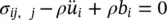
or
(2.20b) 
The second equation is obtained by coupling (2.13) and (2.16) using the definition (2.14) and thus eliminating the variable w i( w). We now have, omitting density changes
(2.21a) 
or
(2.21b) 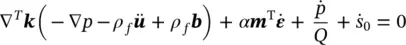
This reduced equation system is precisely the same as that used conventionally in the study of consolidation if the dynamic terms are omitted or even of static problems if the steady state is reached and all the time derivatives are reduced to zero. Thus, the formulation conveniently merges with procedures used for such analyses. However, some loss of accuracy will be evident for problems in which high‐frequency oscillations are important. As we shall show in the next section, these are of little importance for earthquake analyses.
In eliminating the variable w i( w), we have neglected several terms but have achieved an elimination of two or three variable sets depending on whether the two‐ or three‐dimensional problem is considered. However, another possibility exists for obtaining a reduced equation set without neglecting any terms provided that the fluid (i.e. water in this case) is compressible.
With such compressibility assumed, Equation (2.16) can be integrated in time, provided that we introduce the water displacement  in place of the velocity w i( w). We define
(2.22a) 
or
(2.22b) 
where the division by the porosity n is introduced to approximate the true rather than the averaged fluid displacement. We now can rewrite (2.16) after integration with respect to time as
(2.23a) 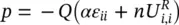
Интервал:
Закладка:
Похожие книги на «Computational Geomechanics»
Представляем Вашему вниманию похожие книги на «Computational Geomechanics» списком для выбора. Мы отобрали схожую по названию и смыслу литературу в надежде предоставить читателям больше вариантов отыскать новые, интересные, ещё непрочитанные произведения.


Обсуждение, отзывы о книге «Computational Geomechanics» и просто собственные мнения читателей. Оставьте ваши комментарии, напишите, что Вы думаете о произведении, его смысле или главных героях. Укажите что конкретно понравилось, а что нет, и почему Вы так считаете.