Savo G. Glisic - Artificial Intelligence and Quantum Computing for Advanced Wireless Networks

Complexity of Instructions

1 Instructions z(t + 1) = z(t) · A + b, 0 = Gw(x, lN), and x(t + 1) = Fw(x(t), l): Since A is a matrix having at most s2 ∣ E∣ nonnull elements, the multiplication of z(t) by A, and as a consequence, the instruction z(t + 1) = z(t) · A + b, costs O(s2 ∣ E∣) floating points operations. The state x (t+1) and the output vector o are calculated by applying the local transition function and the local output function to each node n. Thus, in positional GNNs and in nonlinear GNNs, where fw, hw , and gw are directly implemented by FNNs, x(t + 1) and o are computed by running the forward phase of backpropagation once for each node or edge (see Table 5.2). On the other hand, in linear GNNs, xn(t) is calculated in two steps: the matrices An of Eq. (5.82) and the vectors bn of Eq. (5.83) are evaluated; then, x(t) is computed. The former phase, the cost of which is , is executed once for each epoch, whereas the latter phase, the cost of which is O(s2 ∣ E∣), is executed at every step of the cycle in the function FORWARD.

2 Instruction =(∂Fw/∂x)(x, l): This instruction requires the computation of the Jacobian of Fw. Note that A = {An,u} is a block matrix where the block An,u measures the effect of node u on node n if there is an arc (n,u) from u to n, and is null otherwise. In the linear model, the matrices An,u correspond to those displayed in Eq. (5.82) and are used to calculate x(t) in the forward phase. Thus, such an instruction has no cost in the backward phase in linear GNNs.In nonlinear GNNs, An,u = (∂hw/∂xn)(ln, l(n,u), xu, lu) is computed by appropriately exploiting the backpropagation procedure. In other words, let qi ∈ Rs be a vector where all the components are zero except for the i‐th one, which equals one, that is, q1 = [1, 0, …, 0], q2 = [0, 1, 0, …, 0], and so on. Note that BP, when it is applied to lw with δ = bi, returns , that is, the i‐th column of the Jacobian (∂lw/∂y)(y). Thus, An, u can be computed by applying BP on all the qi, that is,(5.84)

where BP 2indicates that we are considering only the first component of the output of BP. A similar reasoning can also be used with positional GNNs. The complexity of these procedures is easily derived and is displayed in the fourth row of Table 5.2.

1 Computation of ∂ew/∂o and ∂pw/∂w: In linear GNNs, the cost function is , and as a consequence, if nk is a node belonging to the training set, and 0 otherwise. Thus, ∂ew/∂o is easily calculated by O(∣N∣) operations.

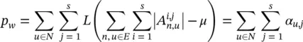
In positional and nonlinear GNNs, a penalty term p wis added to the cost function to force the transition function to be a contraction map. In this case, it is necessary to compute ∂p w/ ∂w , because such a vector must be added to the gradient. Let denote the element in position i , j of the block A n, u. Recalling the definition of p w, we have

where 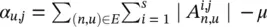if the sum is larger than 0, and 0 otherwise. It follows that

where sgn is the sign function. Let R n, ube a matrix whose element in position i , j is 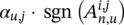, and let vec be the operator that takes a matrix and produces a column vector by stacking all its columns one on top of the other. Then

(5.85)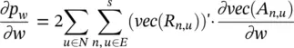

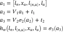
holds. The vector ∂vec( A n, u)/ ∂w depends on selected implementation of h wor f w. For the sake of simplicity, let us restrict our attention to nonlinear GNNs and assume that the transition network is a three‐layered FNN. σ j, a j, V j, and t jare the activation function, the vector of the activation levels, the matrix of the weights, and the thresholds of the j ‐th layer, respectively. σ jis a vectorial function that takes as input the vector of the activation levels of neurons in a layer and returns the vector of the outputs of the neurons of the same layer. The following reasoning can also be extended to positional GNNs and networks with a different number of layers. The function h wis formally defined in terms of σ j, a j, V j, and t j

By the chain differentiation rule, we get

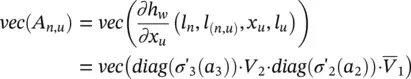
where is the derivative of σ j, diag is an operator that transforms a vector into a diagonal matrix having such a vector as diagonal, and is the submatrix of V 1that contains only the weights that connect the inputs corresponding to x uto the hidden layer. The parameters w affect four components of vec( A n, u), that is, a 3, V 2, a 2, and . By the properties of derivatives for matrix products and the chain rule

(5.86)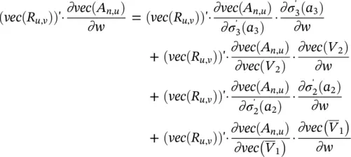

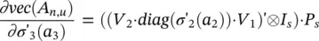
holds. Thus, (vec ( R u,v)) ′· ∂vec( A n,u)/ ∂w is the sum of four contributions. In order to derive a method of computing those terms, let I adenote the a × a identity matrix. Let ⊗ be the Kronecker product, and suppose that P ais a a 2× a matrix such that vec(diag ( v ) = P a v for any vector v ∈ R a. By the Kronecker product’s properties, v e c( AB ) = ( B ′⊗ I a) · v e c( A ) holds for matrices A , B , and I ahaving compatible dimensions [67]. Thus, we have

which implies

Similarly, using the properties vec( ABC ) =( C ′⊗ A ) · vec( B ) and vec( AB ) =( I a⊗ A ) · vec( B ), it follows that