Savo G. Glisic - Artificial Intelligence and Quantum Computing for Advanced Wireless Networks

(5.79)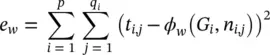

The learning algorithm is based on a gradient‐descent strategy and is composed of the following steps:

1 The states xn(t) are iteratively updated by Eq. (5.78)until at time T they approach the fixed‐point solution of Eq. (5.75): x(T) ≈ x.

2 The gradient ∂ew(T)/∂w is computed.

3 The weights w are updated according to the gradient computed in Step 2.

When it comes to Step 1, note that the hypothesis that F wis a contraction map ensures convergence to the fixed point. Step 3 is carried out within the traditional framework of gradient descent. We will show in the following that Step 3 can be carried out in a very efficient way by exploiting the diffusion process that takes place in GNNs. This diffusion process is very much related to the process that occurs in recurrent neural networks, for which the gradient computation is based on the BPTT algorithm (see Chapter 3). In this case, the encoding network is unfolded from time T back to an initial time t 0. The unfolding produces the layered network shown in Figure 5.10. Each layer corresponds to a time instant and contains a copy of all the units f wof the encoding network. The units of two consecutive layers are connected following graph connectivity. The last layer corresponding to time T also includes the units g wand computes the output of the network.

Backpropagation through time consists of carrying out the traditional backpropagation step (see Chapter 3) on the unfolded network to compute the gradient of the cost function at time T with respect to all the instances of f wand g w. Then, ∂e w( T )/ ∂w is obtained by summing the gradients of all instances. However, backpropagation through time requires storing the states of every instance of the units. When the graphs and T − t 0are large, the memory required may be considerable. On the other hand, in this case, a more efficient approach is possible, based on the Almeida–Pineda algorithm [65, 66]. Since Eq. (5.78)has reached a stable point x before the gradient computation, we can assume that x ( t ) = x holds for any t ≥ t 0. Thus, backpropagation through time can be carried out by storing only x . The following two theorems show that such an intuitive approach has a formal justification. The former theorem proves that function ϕ wis differentiable.

(Differentiability) [1] : Let F wand G wbe the global transition and the global output functions of a GNN, respectively. If F w( x , l ) and G w( x , l N) are continuously differentiable w.r.t. x and w , then ϕ wis continuously differentiable w.r.t. w (for the proof, see [1] ) .

(Backpropagation): Let F wand G wbe the transition and the output functions of a GNN, respectively, and assume that F w( x , l ) and G w( x , l N) are continuously differentiable w.r.t. x and w . Let z ( t ) be defined by

(5.80)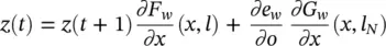

Then, the sequence z ( T ), z ( T − 1)…. . converges to a vector z = lim t → − ∞ z ( t ), and the convergence is exponential and independent of the initial state ( T ). In addition, we have

(5.81)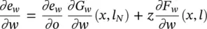

where x is the stable state of the GNN (for the proof, see [1]).

The relationship between the gradient defined by Eq. (5.81)and the gradient computed by the Almeida–Pineda algorithm can be easily recognized. The first term on the right‐hand side of Eq. (5.81)represents the contribution to the gradient due to the output function G w. Backpropagation calculates the first term while it is propagating the derivatives through the layer of the functions g w(see Chapter 3, Figure 3.10). The second term represents the contribution due to the transition function F w. In fact, from Eq. (5.80)

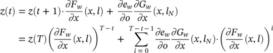
If we assume z ( T ) = ∂e w( T )/ ∂o ( T ) · ( ∂G w/ ∂x ( T ))( x ( T ), l N) and x ( t ) = x , for t 0 ≤ t ≤ T , it follows that

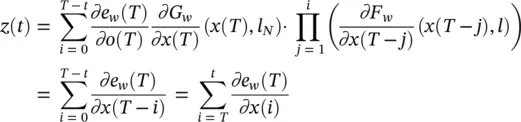
So, Eq. (5.80)accumulates the ∂e w( T )/ ∂x ( i ) into the variable z . This mechanism corresponds to backpropagating the gradients through the layers containing the f wunits. The learning algorithm is detailed in Table 5.1[1]. It consists of a main procedure and of two functions: FORWARD and BACKWARD. The function FORWARD takes as input the current set of parameters w and iterates to find the convergent fixed point. The iteration is stopped when ‖ x ( t ) − x ( t − 1)‖ is less than a given threshold ε faccording to a given norm ‖ · ‖. The function BACKWARD computes the gradient: system Eq. (5.80)is iterated until ‖ z ( t − 1) − z ( t )‖ is smaller than a threshold ε b; then, the gradient is calculated by Eq. (5.81).

The function FORWARD computes the states, whereas BACKWARD calculates the gradient. The procedure MAIN minimizes the error by calling FORWARD and BACKWARD iteratively. Transition and output function implementations : The implementation of the local output function g wdoes not need to fulfill any particular constraint. In GNNs, g wis a multilayered FNN. On the other hand, the local transition function f wplays a crucial role in the proposed model, since its implementation determines the number and the existence of the solutions of Eq. (5.74). The assumption underlying GNN is that the design of f wis such that the global transition function F wis a contraction map with respect to the state x . In the following, we describe two neural network models that fulfill this purpose using different strategies. These models are based on the nonpositional form described by Eq. (5.76). It can be easily observed that there exist two corresponding models based on the positional form as well.

1 Linear (nonpositional) GNN. Eq. (5.76)can naturally be implemented by (5.82)where the vector bn ∈ Rs and the matrix An, u ∈ Rs × s are defined by the output of two FNNs, whose parameters correspond to the parameters of the GNN. More precisely, let us call the transition network an FNN that has to generate An, u and the forcing network another FNN that has to generate bn . Let φw : and ρw : be the functions implemented by the transition and the forcing network, respectively. Then, we define (5.83)where μ ∈ (0, 1) and Θ =resize((φw(ln, l(n, u), lu)) hold, and resize (·) denotes the operator that allocates the elements of an s2‐dimensional vector into an s × s matrix. Thus, An, u is obtained by arranging the outputs of the transition network into the square matrix Θ and by multiplication with the factor μ/s ∣ ne[u]∣. On the other hand, bn is just a vector that contains the outputs of the forcing network. In the following, we denote the 1‐norm of a matrix M = {mi, j} as ‖M‖1 = maxj ∑ ∣ mi, j∣ and assume that ‖φw(ln, l(n, u), lu)‖1 ≤ s holds; this can be straightforwardly verified if the output neurons of the transition network use an appropriately bounded activation function, for example, a hyperbolic tangent.