Savo G. Glisic - Artificial Intelligence and Quantum Computing for Advanced Wireless Networks

where Gconv (·) is a graph convolutional layer. The Graph Convolutional Recurrent Network (GCRN) combines a LSTM network with ChebNet. DCRNN incorporates a proposed DGC layer ( Eq. (5.50)) into a GRU network.

Previous methods all use a predefined graph structure. They assume the predefined graph structure reflects the genuine dependency relationships among nodes. However, with many snapshots of graph data in a spatial‐temporal setting, it is possible to learn latent static graph structures automatically from data. To realize this,

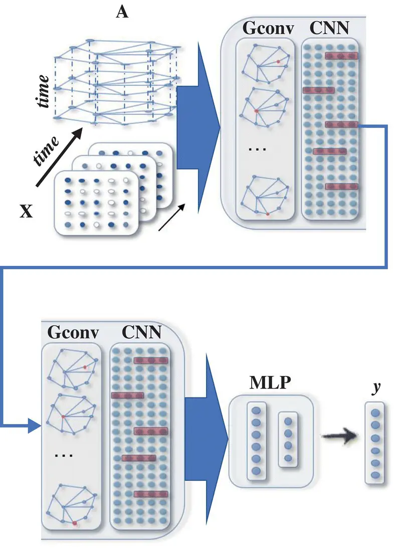
Figure 5.7 A STGNN for spatial‐temporal graph forecasting. A graph convolutional layer is followed by a 1D‐CNN layer. The graph convolutional layer operates on A and X(t) to capture the spatial dependency, while the 1D‐CNN layer slides over X along the time axis to capture the temporal dependency. The output layer is a linear transformation, generating a prediction for each node, such as its future value at the next time step.

Source: Wu et al. [38].

Graph WaveNet [61] proposes a self‐adaptive adjacency matrix to perform graph convolutions. The self‐adaptive adjacency matrix is defined as

(5.72)

where the softmax function is computed along the row dimension, E1 denotes the source node embedding, and E2 denotes the target node embedding with learnable parameters. By multiplying E1 with E2, one can get the dependency weight between a source node and a target node. With a complex CNN‐based spatial‐temporal neural network, Graph WaveNet performs well without being given an adjacency matrix.

In order to analyze the network complexity, we need a more detailed definition of both network topologies and network parameters. For this, we will use the original definitions introduced in [1], one of the first papers in this field. For this reason, in this section we will revisit the description of the GNN with more details on the specific model of the network, computation of the states, the learning process, and specific transition and output function implementations, and to facilitate a better understanding of these processes, we will provide a comparison with random walks and recursive neural nets. When discussing computational complexity issues, we will look at the complexity of instructions and the time complexity of the GNN mode. The illustrations will be based on the results presented in [1].

Here, a graph G is a pair ( N , E ), where N is the set of nodes and E is the set of edges. The set n e [ n ] stands for the neighbors of n , that is, the nodes connected to n by an arc, while co[ n ] denotes the set of arcs having n as a vertex. Nodes and edges may have labels represented by real vectors. The labels attached to node n and edge ( n 1, n 2) will be represented by and , respectively. Let l denote the vector obtained by stacking together all the labels of the graph.

If y is a vector that contains data from a graph and S is a subset of the nodes (the edges), then y Sdenotes the vector obtained by selecting from y the components related to the node (the edges) in S .

For example, l ne[n]stands for the vector containing the labels of all the neighbors of n . Labels usually include features of objects related to nodes and features of the relationships between the objects. No assumption is made regarding the arcs: directed and undirected edges are both permitted. However, when different kinds of edges coexist in the same dataset, it is necessary to distinguish them. This can be easily achieved by attaching a proper label to each edge. In this case, different kinds of arcs turn out to be just arcs with different labels.

The considered graphs may be either positional or nonpositional. Nonpositional graphs are those that have been described thus far; positional graphs differ from them since a unique integer identifier is assigned to each neighbor of a node n to indicate its logical position. Formally, for each node n in a positional graph, there exists an injective function ν n: ne[ n ] → {1, …, ∣ N∣}, which assigns to each neighbor u of n a position ν n( u ).

The domain is the set of pairs of a graph and a node, that is, , where is a set of the graphs and is a subset of their nodes. We assume a supervised learning framework with the learning set

(5.73)

where n i, j∈ N idenotes the j ‐th node in the set and t i, jis the desired target associated with n i, j. Finally, and q i≤ ∣ N i∣. All the graphs of the learning set can be combined into a unique disconnected graph, and therefore one might think of the learning set as the pair , where G = ( N , E ) is a graph and is a set of pairs {( n i, t i) ∣ n i∈ N , t i∈ R m, 1 ≤ i ≤ q }. It is worth mentioning that this compact definition is useful not only for its simplicity, but that it also directly captures the very nature of some problems where the domain consists of only one graph, for instance, a large portion of the Web (see Figure 5.8).

The model: As before, the nodes in a graph represent objects or concepts, and edges represent their relationships. Each concept is naturally defined by its features and the related concepts. Thus, we can attach a state x n∈ R sto each node n that is based on the information contained in the neighborhood of n (see Figure 5.9). The state x ncontains a representation of the concept denoted by n and can be used to produce an output o, that is, a decision about the concept. Let f wbe a parametric function, called the local transition function , that expresses the dependence of a node n on its neighborhood, and let g wbe the local output function that describes how the output is produced. Then, x nand o nare defined as follows: