Savo G. Glisic - Artificial Intelligence and Quantum Computing for Advanced Wireless Networks
Здесь есть возможность читать онлайн «Savo G. Glisic - Artificial Intelligence and Quantum Computing for Advanced Wireless Networks» — ознакомительный отрывок электронной книги совершенно бесплатно, а после прочтения отрывка купить полную версию. В некоторых случаях можно слушать аудио, скачать через торрент в формате fb2 и присутствует краткое содержание. Жанр: unrecognised, на английском языке. Описание произведения, (предисловие) а так же отзывы посетителей доступны на портале библиотеки ЛибКат.

- Название:Artificial Intelligence and Quantum Computing for Advanced Wireless Networks
- Автор:
- Жанр:
- Год:неизвестен
- ISBN:нет данных
- Рейтинг книги:3 / 5. Голосов: 1
-
Избранное:Добавить в избранное
- Отзывы:
-
Ваша оценка:
Artificial Intelligence and Quantum Computing for Advanced Wireless Networks: краткое содержание, описание и аннотация
Предлагаем к чтению аннотацию, описание, краткое содержание или предисловие (зависит от того, что написал сам автор книги «Artificial Intelligence and Quantum Computing for Advanced Wireless Networks»). Если вы не нашли необходимую информацию о книге — напишите в комментариях, мы постараемся отыскать её.
A practical overview of the implementation of artificial intelligence and quantum computing technology in large-scale communication networks Artificial Intelligence and Quantum Computing for Advanced Wireless Networks
Artificial Intelligence and Quantum Computing for Advanced Wireless Networks
Artificial Intelligence and Quantum Computing for Advanced Wireless Networks — читать онлайн ознакомительный отрывок
Ниже представлен текст книги, разбитый по страницам. Система сохранения места последней прочитанной страницы, позволяет с удобством читать онлайн бесплатно книгу «Artificial Intelligence and Quantum Computing for Advanced Wireless Networks», без необходимости каждый раз заново искать на чём Вы остановились. Поставьте закладку, и сможете в любой момент перейти на страницу, на которой закончили чтение.
Интервал:
Закладка:
where MLP (·) represents a multi‐layer perceptron. As the number of neighbors of a node can vary from one to a thousand or even more, it is inefficient to take the full size of a node’s neighborhood. GraphSAGE [23] adopts sampling to obtain a fixed number of neighbors for each node. It performs graph convolutions by
(5.56) 
where  f k(·) is an aggregation function, S N(v)is a random sample of the node v ’s neighbors. The aggregation function should be invariant to the permutations of node orderings such as a mean, sum, or max function.
GAT [53] assumes that contributions of neighboring nodes to the central node are neither identical like GraphSAGE [23], nor pre‐determined like GCN [14]. GAT adopts attention mechanisms to learn the relative weights between two connected nodes. The graph convolutional operation according to GAT is defined as
(5.57) 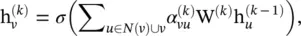
where  . The attention weight
  measures the connective strength between the node v and its neighbor u :
(5.58) 
where g (·) is a LeakyReLU activation function and a is a vector of learnable parameters. The softmax function ensures that the attention weights sum up to one over all neighbors of the node v .
Graph pooling modules : After a GNN generates node features, we can use them for the final task. But using all these features directly can be computationally challenging, and thus a downsampling strategy is needed. Depending on the objective and the role it plays in the network, different names are given to this strategy: (i) the pooling operation aims to reduce the size of parameters by downsampling the nodes to generate smaller representations and thus avoid overfitting, permutation invariance, and computational complexity issues and (ii) the readout operation is mainly used to generate graph‐level representation based on node representations (see Figure 5.5). Their mechanism is very similar. In this section, we use pooling to refer to all kinds of downsampling strategies applied to GNNs. Nowadays, mean/max/sum pooling, already illustrated in Section 5.1, is the most primitive and effective way to implement downsampling since calculating the mean/ max /sum value in the pooling window is fast:
(5.59) 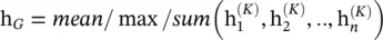
where K is the index of the last graph convolutional layer.
5.2.3 Graph Autoencoders (GAEs)
These are deep neural architectures that map nodes into a latent feature space and decode graph information from latent representations. GAEs can be used to learn network embeddings or generate new graphs.
Network embedding (encoding) is a low‐dimensional vector representation of a node that preserves a node’s topological information. GAEs learn network embeddings using an encoder to extract network embeddings and using a decoder to enforce network embeddings to preserve the graph topological information such as the PPMI matrix and the adjacency matrix (see Figure 5.6).
Earlier approaches mainly employ multi‐layer perceptrons to build GAEs for network embedding learning. Deep Neural Network for Graph Representations (DNGR) uses a stacked denoising autoencoder to encode and decode the PPMI matrix via multi‐layer perceptrons. Concurrently, Structural Deep Network Embedding (SDNE) uses a stacked autoencoder to jointly preserve the node first‐order proximity and second‐order proximity. SDNE proposes two loss functions on the outputs of the encoder and the outputs of the decoder separately. The first loss function enables the learned network embeddings to preserve the node’s first‐order proximity by minimizing the distance between a node’s network embedding and its neighbors’ network embeddings. The first loss function L 1stis defined as
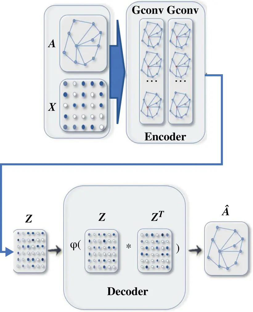
Figure 5.6 A graph autoencoder (GAE) for network embedding. The encoder uses graph convolutional layers to get a network embedding for each node. The decoder computes the pairwise distance given network embeddings. After applying a nonlinear activation function, the decoder reconstructs the graph adjacency matrix. The network is trained by minimizing the discrepancy between the real adjacency matrix and the reconstructed adjacency matrix.
Source: Wu et al. [38].
(5.60) 
where x v= A v, :and enc (·) is an encoder that consists of a multi‐layer perceptron. The second loss function enables the learned network embeddings to preserve the node’s second‐order proximity by minimizing the distance between a node’s inputs and its reconstructed inputs and is defined as
(5.61) 
where b v, u= 1 if A v, u= 0, b v, u= β > 1 if A v, u= 1, and dec (·) is a decoder that consists of a multi‐layer perceptron.
DNGR [54] and SDNE [55] only consider node structural information about the connectivity between pairs of nodes. They ignore the fact that the nodes may contain feature information that depicts the attributes of nodes themselves. Graph Autoencoder (GAE*) [56] leverages GCN [14] to encode node structural information and node feature information at the same time. The encoder of GAE* consists of two graph convolutional layers, which takes the form
(5.62) 
where Z denotes the network embedding matrix of a graph, f (·) is a ReLU activation function, and the Gconv (·) function is a graph convolutional layer defined by Eq. (5.44). The decoder of GAE* aims to decode node relational information from their embeddings by reconstructing the graph adjacency matrix, which is defined as
(5.63) 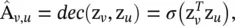
Интервал:
Закладка:
Похожие книги на «Artificial Intelligence and Quantum Computing for Advanced Wireless Networks»
Представляем Вашему вниманию похожие книги на «Artificial Intelligence and Quantum Computing for Advanced Wireless Networks» списком для выбора. Мы отобрали схожую по названию и смыслу литературу в надежде предоставить читателям больше вариантов отыскать новые, интересные, ещё непрочитанные произведения.


Обсуждение, отзывы о книге «Artificial Intelligence and Quantum Computing for Advanced Wireless Networks» и просто собственные мнения читателей. Оставьте ваши комментарии, напишите, что Вы думаете о произведении, его смысле или главных героях. Укажите что конкретно понравилось, а что нет, и почему Вы так считаете.