Savo G. Glisic - Artificial Intelligence and Quantum Computing for Advanced Wireless Networks

Chebyshev Spectral CNN ( ChebNet ) [45] approximates the filter g θby Chebyshev polynomials of the diagonal matrix of eigenvalues, that is, 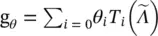, where 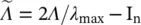, and the values of lie in [−1, 1]. The Chebyshev polynomials are defined recursively by T i(x) = 2x T i − 1(x) − T i − 2(x) with T 0(x) = 1 and T 1(x) = x. As a result, the convolution of a graph signal x with the defined filter g θis

(5.39)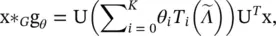

where 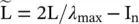. As 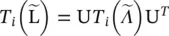, which can be proved by induction on i . ChebNet takes the form

(5.40)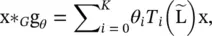

As an improvement over spectral CNN, the filters defined by ChebNet are localized in space, which means filters can extract local features independently of the graph size. The spectrum of ChebNet is mapped to [−1, 1] linearly. CayleyNet [47] further applies Cayley polynomials, which are parametric rational complex functions, to capture narrow frequency bands. The spectral graph convolution of CayleyNet is defined as

(5.41)

where Re (·) returns the real part of a complex number, c 0is a real coefficent, c jis a complex coefficent, i is the imaginary number, and h is a parameter that controls the spectrum of a Cayley filter. While preserving spatial locality, CayleyNet shows that ChebNet can be considered as a special case of CayleyNet.

GCN [14] introduces a first‐order approximation of ChebNet. Assuming K = 1 and λ max= 2, Eq. (5.40)is simplified as

(5.42)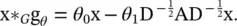

To restrict the number of parameters and avoid overfitting, GCN further assume θ = θ 0= − θ 1, leading to the following definition of a graph convolution:

(5.43)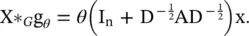

To allow multi‐channels of inputs and outputs, GCN modifies Eq. (5.43)into a compositional layer, defined as

(5.44)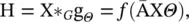

where and f (·) is an activation function. Using empirically causes numerical instability to GCN. To address this problem, GCN applies a normalization to replace by with and 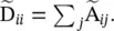Being a spectral‐based method, GCN can be also interpreted as a spatial‐based method. From a spatial‐based perspective, GCN can be considered as aggregating feature information from a node’s neighborhood. Equation (5.44)can be expressed as

(5.45)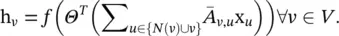

Several recent works made incremental improvements over GCN [14] by exploring alternative symmetric matrices.

Adaptive Graph Convolutional Network ( AGCN ) [16] learns hidden structural relations unspecified by the graph adjacency matrix. It constructs a so‐called residual graph adjacency matrix through a learnable distance function that takes two nodes’ features as inputs.

DGCN [17] introduces a dual graph convolutional architecture with two graph convolutional layers in parallel. While these two layers share parameters, they use the normalized adjacency matrix and the PPMI matrix, which capture nodes’ co‐occurrence information through random walks sampled from a graph. The PPMI matrix is defined as

(5.46)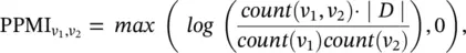

where v 1, v 2∈ V , ∣ D ∣ 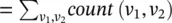, and the count (·) function returns the frequency with which node v and/or node u co‐occur/occur in sampled random walks. By ensembling outputs from dual graph convolutional layers, DGCN encodes both local and global structural information without the need to stack multiple graph convolutional layers.

Spatial ‐ based ConvGNNs : Analogous to the convolutional operation of a conventional CNN on an image, spatial‐based methods define graph convolutions based on a node’s spatial relations. Images can be considered as a special form of graph with each pixel representing a node. Each pixel is directly connected to its nearby pixels, as illustrated in Figure 5.3a (adopted from [38]). A filter is applied to a 3 × 3 patch by taking the weighted average of pixel values of the central node and its neighbors across each channel. Similarly, the spatial‐based graph convolutions convolve the central node’s representation with its neighbors’ representations to derive the updated representation for the central node, as illustrated in Figure 5.3b. From another perspective, spatial‐based ConvGNNs share the same idea of information propagation/message passing with RecGNNs. The spatial graph convolutional operation essentially propagates node information along edges.