Savo G. Glisic - Artificial Intelligence and Quantum Computing for Advanced Wireless Networks

GN block contains three “update” functions, φ, and three “aggregation” functions, ρ ,

(5.32)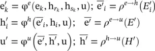

where 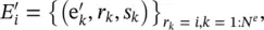, and . The ρ functions must be invariant to permutations of their inputs and should take variable numbers of arguments.

The computation steps of a GN block:

1 φe is applied per edge, with arguments (, ,u), and returns . The set of resulting per‐edge outputs for each node i is, = , and is the set of all per‐edge outputs.

2 ρe → h is applied to , and aggregates the edge updates for edges that project to vertex i, into which will be used in the next step’s node update.

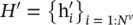
3 φh is applied to each node i, to compute an updated node attribute, . The set of resulting per‐node outputs is .

4 ρe → u is applied to E′, and aggregates all edge updates, into , which will then be used in the next step’s global update.

5 ρh → u is applied to H′, and aggregates all node updates, into , which will then be used in the next step’s global update.

6 φu is applied once per graph and computes an update for the global attribute, u′.

In the previous section, we have briefly surveyed a number of GNN designs with the very basic description of their principles. Here, we categorize these options into recurrent graph neural networks ( RecGNNs ), convolutional graph neural networks ( ConvGNNs ), graph autoencoders ( GAEs ), and spatial‐temporal graph neural networks ( STGNNs ) and provide more details about their operations.

Figures 5.2– 5.5, inspired by [38], give examples of various model architectures. In the following, we provide more information for each category, mainly on computation of the state, the learning algorithm , and transition and output function implementations .

These networks go back to the beginnings of GNNs. They apply the same set of parameters recurrently over nodes in a graph to extract high‐level node representations. Limited by computational power, earlier research mainly focused on directed acyclic graphs, while later works extended these models to handle general types of graphs, for example, acyclic, cyclic, directed, and undirected graphs [1]. Based on an information diffusion mechanism, this particular GNN (in the sequel referred to as GNN*) updates nodes’ states by exchanging neighborhood information recurrently until a stable equilibrium is reached. A node’s hidden state is recurrently updated by

(5.33)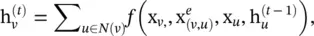

where f (·) is a parametric function, and is initialized randomly. The sum operation enables GNN* to be applicable to all nodes, even if the number of neighbors differs and no neighborhood ordering is known. To ensure convergence, the recurrent function f (·) must be a contraction mapping, which shrinks the distance between two points after projecting them into a latent space. If f (·) is a neural network, a penalty term has to be imposed on the Jacobian matrix of parameters. When a convergence criterion is satisfied, the last step node’s hidden states are forwarded to a readout layer. GNN* alternates the stage of node state propagation and the stage of parameter gradient computation to minimize a training objective. This strategy enables GNN to handle cyclic graphs.

Graph Echo State Network ( GraphESN ) , developed in follow‐up works [40], extends echo state networks to improve the training efficiency of GNN*. GraphESN consists of an encoder and an output layer. The encoder is randomly initialized and requires no training. It implements a contractive state transition function to recurrently update node states until the global graph state reaches convergence. Afterward, the output layer is trained by taking the fixed node states as inputs.

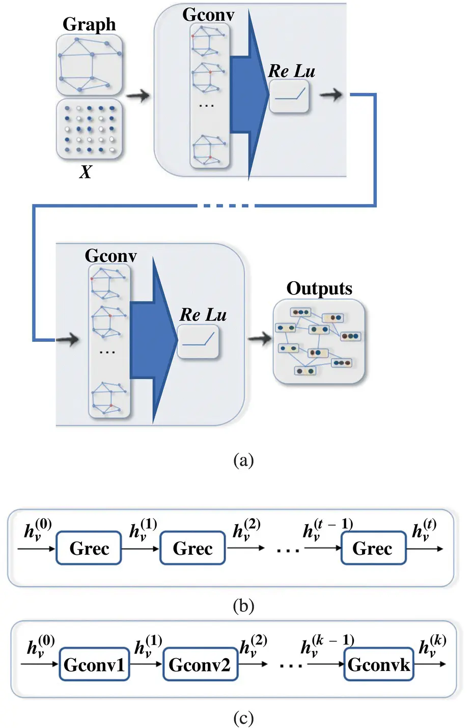
Figure 5.2 Illustrations of ConvGNN network: (a) A ConvGNN with multiple graph convolutional layers. A graph convolutional layer encapsulates each node’s hidden representation by aggregating feature information from its neighbors. After feature aggregation, a nonlinear transformation is applied to the resulted outputs. By stacking multiple layers, the final hidden representation of each node receives messages from a further neighborhood. (b) Recurrent Graph Neural Networks (RecGNNs) use the same graph recurrent layer (Grec) to update node representations. (c) Convolutional Graph Neural Networks (ConvGNNs) use a different graph convolutional layer (Gconv) to update node representations.

Source: Wu et al. [38].

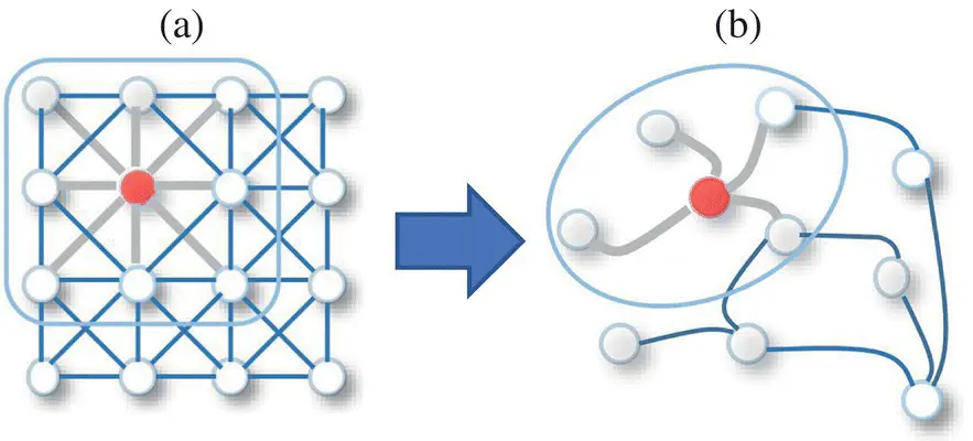
Figure 5.3 2D Convolution versus graph convolution: (a) 2D convolution. Analogous to a graph, each pixel in an image is taken as a node where neighbors are determined by the filter size. The 2D convolution takes the weighted average of pixel values of the gray node along with its neighbors. The neighbors of a node are ordered and have a fixed size. (b) Graph convolution. To get a hidden representation of the gray node, one simple solution of the graph convolutional operation is to take the average value of the node features of the gray node along with its neighbors. Unlike image data, the neighbors of a node are unordered and variable in size.

Source: Wu et al. [38].

GGNN [41] employs a GRU [42] as a recurrent function, reducing the recurrence to a fixed number of steps. The advantage is that it no longer needs to constrain parameters to ensure convergence. A node’s hidden state is updated by its previous hidden states and its neighboring hidden states, defined as

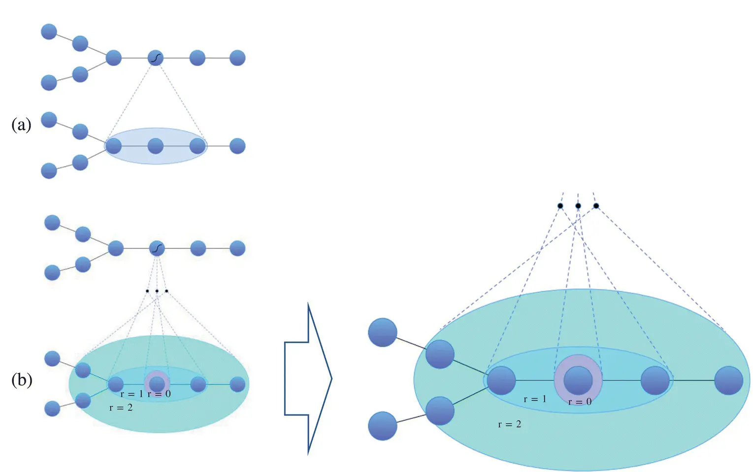
Figure 5.4 Parametric graph convolution: (a) Conventional graph convolutional concept. (b) Parametric graph convolution, where r controls the maximum distance of the considered neighborhood, and the dimensionality of the output [39].

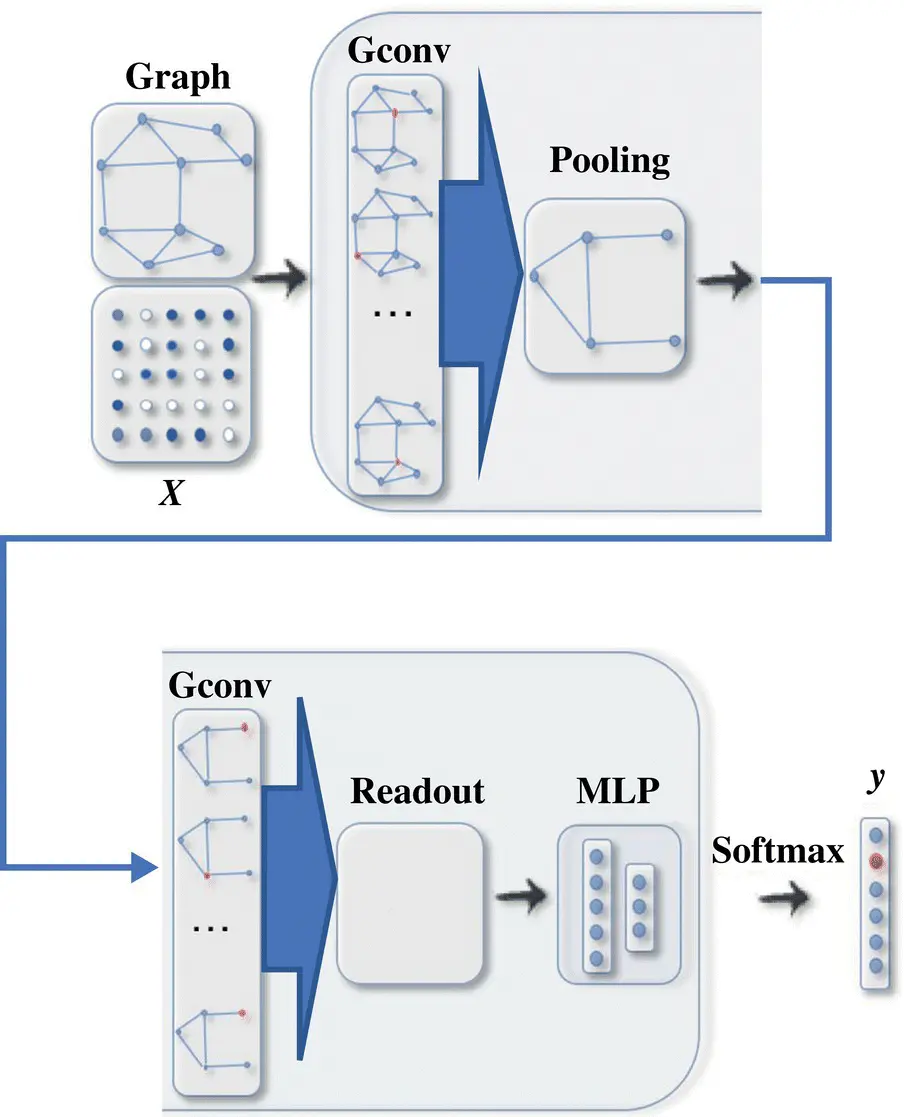
Figure 5.5 A ConvGNN with pooling and readout layers for graph classification. A graph convolutional layer is followed by a pooling layer to coarsen a graph into subgraphs so that node representations on coarsened graphs represent higher graph‐level representations. A readout layer summarizes the final graph representation by taking the sum/mean of hidden representations of subgraphs.