Savo G. Glisic - Artificial Intelligence and Quantum Computing for Advanced Wireless Networks

(5.11)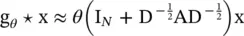

Non‐spectral approaches define convolutions directly on the graph, operating on spatially close neighbors. The major challenge with non‐spectral approaches is defining the convolution operation with differently sized neighborhoods and maintaining the local invariance of CNNs.

Neural fingerprints ( FP ) [15] use different weight matrices for nodes with different degrees,

(5.12)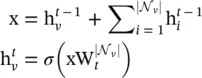

where is the weight matrix for nodes with degree at layer t . The main drawback of the method is that it cannot be applied to large‐scale graphs with more node degrees.

Diffusion‐convolutional neural networks ( DCNNs ) were proposed in [16].Transition matrices are used to define the neighborhood for nodes in DCNN. For node classification, it has the form

(5.13)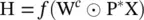

where X is an N × F tensor of input features ( N is the number of nodes, and F is the number of features). P *is an N × K × N tensor that contains the power series {P, P 2, …, P K} of matrix P, and P is the degree‐normalized transition matrix from the graph adjacency matrix A. Each entity is transformed to a diffusion convolutional representation that is a K × F matrix defined by K hops of graph diffusion over F features. It will then be defined by a K × F weight matrix and a nonlinear activation function f . Finally, H (which is N × K × F ) denotes the diffusion representations of each node in the graph. As for graph classification, DCNN simply takes the average of nodes’ representation,

(5.14)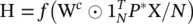

and 1 Nhere is an N × 1 vector of ones. DCNN can also be applied to edge classification tasks, which requires converting edges to nodes and augmenting the adjacency matrix.

Dual graph convolutional network ( DGCN) [17]: This jointly considers the local consistency and global consistency on graphs. It uses two convolutional networks to capture the local/global consistency and adopts an unsupervised loss function to ensemble them. As the first step, let us note that stacking the operator in Eq. (5.11)could lead to numerical instabilities and exploding/vanishing gradients, so [14] introduces the renormalization trick : 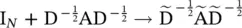, with and . Finally, [14] generalizes the definition to a signal X ∈ ℝ N × Cwith C input channels and F filters for feature maps as follows:

(5.15)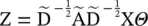

where Θ ∈ ℝ C × Fis a matrix of filter parameters, and Z ∈ ℝ N × Fis the convolved signal matrix. The first convolutional network for DGCN is the same as Eq. (5.15). The second network replaces the adjacency matrix with a positive pointwise mutual information (PPMI) matrix:

(5.16)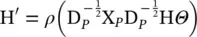

where X Pis the PPMI matrix, and D Pis the diagonal degree matrix of X P.

When dealing with large‐scale networks, low‐dimensional vector embeddings of nodes in large graphs have proved extremely useful as feature inputs for a wide variety of prediction and graph analysis tasks [18–22]. The basic idea behind node‐embedding approaches is to use dimensionality reduction techniques to distill the high‐dimensional information about a node’s graph neighborhood into a dense vector embedding. These node embeddings can then be fed to downstream machine learning systems and aid in tasks such as node classification, clustering, and link prediction [19–21].

GraphSAGE (SAmple and aggreGatE) [23] is a general inductive framework. The framework generates embeddings by sampling and aggregating features from a node’s local neighborhood.

(5.17)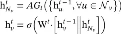

However, the original work utilizes in Eq. (5.17)only a fixed‐size set of neighbors by uniformly sampling. Three aggregator functions are used.

The mean aggregator could be viewed as an approximation of the convolutional operation from the transductive GCN framework [14], so that the inductive version of the GCN variant could be derived by

(5.18)

The mean aggregator is different from other aggregators because it does not perform the concatenation operation that concatenates and in Eq. (5.17). It could be viewed as a form of “skip connection” [24] and could achieve better performance.

The long short‐term memory ( LSTM ) aggregator , which has a larger expressive capability, is also used. However, LSTMs process inputs in a sequential manner so that they are not permutation invariant. Reference [23] adapts LSTMs to operate on an unordered set by permutating the node’s neighbors.

Pooling aggregator: In the pooling aggregator, each neighbor’s hidden state is fed through a fully connected layer, after which a max ‐pooling operation is applied to the set of the node’s neighbors:

(5.19)