Savo G. Glisic - Artificial Intelligence and Quantum Computing for Advanced Wireless Networks

Note that any symmetric function could be used in place of the max ‐pooling operation here. The operation of GraphSAGE is illustrated in Figure 5.1[23].

Gate: Several works have attempted to use a gate mechanism such as gate recurrent units (GRUs) [25] or LSTM [26] in the propagation step to mitigate the restrictions in the former GNN models and improve the long‐term propagation of information across the graph structure.

Gated graph neural network ( GGNN ) [27] uses GRUs in the propagation step, unrolls the recurrence for a fixed number of steps T , and uses backpropagation through time in order to compute gradients. So, the propagation model can be presented as

(5.20)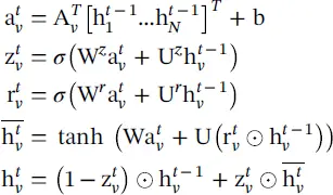

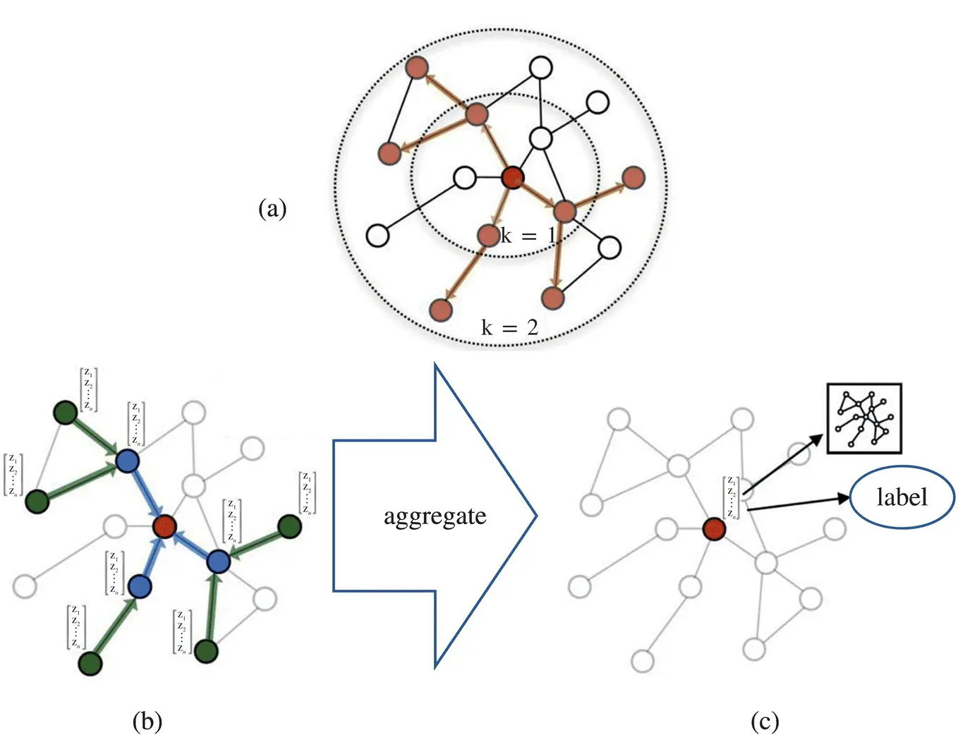
Figure 5.1 Operation of GraphSAGE: (a) sample neighborhood, (b) aggregate feature information from neighbors, (c) predict graph context and label using aggregated information.

Source: Hamilton et al. [23].

The node v first aggregates message from its neighbors, where A vis the submatrix of the graph adjacency matrix A and denotes the connection of node v with its neighbors. The GRU‐like update functions incorporate information from the other nodes and from the previous time step to update each node’s hidden state. Matrix a gathers the neighborhood information of node v , and z and r are the update and reset gates.

LSTM architecture extensions , referred to as the Child ‐ Sum Tree‐LSTM and the N ‐ ary Tree‐LSTM , are presented in [28]. As in standard LSTM units, each Tree‐LSTM unit (indexed by v ) contains input and output gates i vand o v, a memory cell c v, and a hidden state h v. Instead of a single forget gate, the Tree‐LSTM unit contains one forget gate f vkfor each child k , allowing the unit to selectively incorporate information from each child. The Child‐Sum Tree‐LSTM transition equations are given as

(5.21)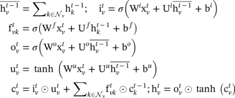

is the input vector at time t in the standard LSTM setting. If the branching factor of a tree is at most K and all children of a node are ordered, – that is, they can be indexed from 1 to K – then the N ‐ary Tree‐LSTM can be used. For node v , and denote the hidden state and memory cell of its k ‐th child at time t , respectively. The transition equations are now

(5.22)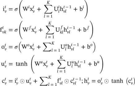

The introduction of separate parameter matrices for each child k allows the model to learn more fine‐grained representations conditioning on the states of a unit’s children than the Child‐Sum Tree‐LSTM.

The two types of Tree‐LSTMs can be easily adapted to the graph. The graph‐structured LSTM in [29] is an example of the N ‐ary Tree‐LSTM applied to the graph. However, it is a simplified version since each node in the graph has at most two incoming edges (from its parent and sibling predecessor). Reference [30] proposed another variant of the Graph LSTM based on the relation extraction task. The main difference between graphs and trees is that edges of graphs have labels. Work in [30] utilizes different weight matrices to represent different labels:

(5.23)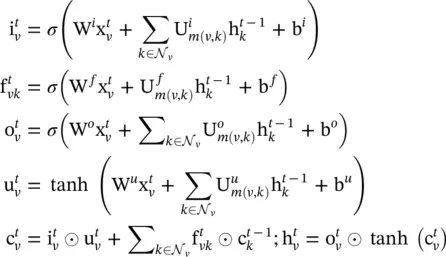

where m ( v , k ) denotes the edge label between node v and k .

The attention mechanism has been successfully used in many sequence‐based tasks such as machine translation [31–33] and machine reading [34]. Work in [35] proposed a graph attention network (GAT) that incorporates the attention mechanism into the propagation step. It computes the hidden states of each node by attending to its neighbors, following a self ‐ attention strategy. The work defines a single graph attentional layer and constructs arbitrary GATs by stacking this layer. The layer computes the coefficients in the attention mechanism of the node pair ( i , j ) by

(5.24)

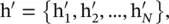
where α ijis the attention coefficient of node j to represents the neighborhoods of node i in the graph. The input set of node features to the layer is h = {h 1, h 2, …, h N}, h i∈ ℝ F, where N is the number of nodes, and F is the number of features of each node; the layer produces a new set of node features (of potentially different cardinality F ′), , as its output. is the weight matrix of a shared linear transformation that is applied to every node, and is the weight vector of a single‐layer FNN. It is normalized by a softmax function, and the LeakyReLU nonlinearity (with negative input slope α = 0.2) is applied. After applying a nonlinearity, the final output features of each node can be obtained as

(5.25)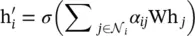

The layer utilizes multi ‐ head attention similarly to [33] to stabilize the learning process. It applies K independent attention mechanisms to compute the hidden states and then concatenates their features (or computes the average), resulting in the following two output representations: