Savo G. Glisic - Artificial Intelligence and Quantum Computing for Advanced Wireless Networks

84 84 Bach, S., Binder, A., Montavon, G. et al. (2015). On pixel‐wise explanations for non‐linear classifier decisions by layer‐wise relevance propagation. PLoS One 10 (7): e0130140.

85 85 A. Fisher, C. Rudin, and F. Dominici. (2018). “Model class reliance: Variable importance measures for any machine learning model class, from the ‘rashomon’ perspective.” [Online]. Available: https://arxiv.org/abs/1801.01489

86 86 Bien, J. and Tibshirani, R. (2011). Prototype selection for interpretable classification. Ann. Appl. Statist. 5 (4): 2403–2424.

87 87 B. Kim, C. Rudin, and J. A. Shah, “The Bayesian case model: A generative approach for case‐based reasoning and prototype classification,” in Proc. Adv. Neural Inf. Process. Syst., 2014, pp. 1952–1960.

88 88 K. S. Gurumoorthy, A. Dhurandhar, and G. Cecchi. (2017). “ProtoDash: Fast interpretable prototype selection.” [Online]. Available: https://arxiv.org/abs/1707.01212

89 89 B. Kim, R. Khanna, and O. O. Koyejo, “Examples are not enough, learn to criticize! criticism for interpretability,” in Proc. 29th Conf. Neural Inf. Process. Syst. (NIPS), 2016, pp. 2280–2288.

90 90 S. Wachter, B. Mittelstadt, and C. Russell. (2017). “Counterfactual explanations without opening the black box: Automated decisions and the GDPR.” [Online]. Available: https://arxiv.org/abs/1711.00399

91 91 X. Yuan, P. He, Q. Zhu, and X. Li. (2017). “Adversarial examples: Attacks and defenses for deep learning.” [Online]. Available: https://arxiv.org/abs/1712.07107

92 92 G. Montavon, S. Bach, A. Binder, W. Samek, and K.‐R. Muller Explaining NonLinear Classification Decisions with Deep Taylor Decomposition, arXiv:1512.02479v1 [cs.LG] 8 Dec 2015, also in Pattern Recognition, vol. 65 May 2017, Pages pp. 211–222.

93 93 W. J. Murdoch, A. Szlam, Automatic Rule Extraction from Long Short Term Memory Networks, ICLR 2017 Conference

94 94 R. Babuska, Fuzzy Systems, Modeling and Identification https://www.researchgate.net/profile/Robert_Babuska/publication/228769192_Fuzzy_Systems_Modeling_and_Identification/links/02e7e5223310e79d19000000/Fuzzy‐Systems‐Modeling‐and‐Identification.pdf

95 95 Glisic, S. (2016). Advanced Wireless Networks: Technology and Business Models. Wiley.

96 96 B. E. Boser, I. Guyon, V. N. Vapnik A training algorithm for optimal margin classifiers. In D. Haussler, editor, Proceedings of the Annual Conference on Computational Learning Theory, pages 144–152, Pittsburgh, PA, 1992. ACM Press.

97 97 Chan, W.C. et al. (2001). On the modeling of nonlinear dynamic systems using support vector neural networks. Eng. Appl. Artif. Intel. 14 (2): 105–113.

98 98 Chiang, J.H. and Hao, P.Y. (2004). Support vector learning mechanism for fuzzy rule‐based modeling: a new approach. IEEE Trans. Fuzzy Syst. 12 (1): 1–12.

99 99 Shen, J., Syau, Y., and Lee, E.S. (2007). Support vector fuzzy adaptive network in regression analysis. Comput. Math. Appl. 54 (11–12): 1353–1366.

100 100 Smola, A.J. and Schölkopf, B. (1998). The connection between regularization operators and support vector kernels. Neural Netw. 10: 1445–1454.

101 101 https://en.wikipedia.org/wiki/T‐norm:fuzzy_logics

102 102 https://en.wikipedia.org/wiki/Construction_of_t‐norms

103 103 Cherkassky, V. and Ma, Y. (2004). Practical selection of SVM parameters and noise estimation for SVM regression. Neural Netw. 17 (1): 113–126.

104 104 Chalimourda, A., Schölkopf, B., and Smola, A.J. (2004). Experimentally optimal v in support vector regression for different noise models and parameters settings. Neural Netw. 17 (1): 127–141.

105 105 Yu, L. and Xiao, J. (2009). Trade‐off between accuracy and interpretability: experience‐oriented fuzzy modeling via reduced‐set vectors. Comput. Math. Appl. 57: 885–895.

As a start, in this section we present a brief overview of the and then in the subsequent sections discuss some of the most popular variants in more detail.

The basic idea here is to extend existing neural networks for the purpose of processing the data represented in graph domains [1]. In a graph, each node is defined by its own features and the features of the related nodes. The target of GNN is to learn a state embedding h v∈ ℝ sthat contains information on the neighborhood for each node. The state embedding h vis an s ‐dimension vector of node v and can be used to produce an output o v. Let f be a parametric function, called the local transition function , that is shared among all nodes and updates the node state according to the input neighborhood. Let g be the local output function that describes how the output is produced. Then, h vand o vare defined as

(5.1)

where x v, x co[v], h ne[v], and x ne[v]are the features of v , the features of its edges, the states, and the features of the nodes in the neighborhood of v , respectively. If H, O, X, and X Nare the vectors constructed by stacking all the states, all the outputs, all the features, and all the node features, respectively, then we can write

(5.2)

In Eq. (5.2), F , the global transition function , and G , the global output function , are stacked versions of f and g for all nodes in a graph, respectively. The value of H is the fixed point of Eq. (5.2)and is uniquely defined with the assumption that F is a contraction map. GNN uses the following iterative scheme for computing the state (Banach’s fixed‐point theorem [2])

(5.3)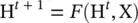

where H tdenotes the t ‐th iteration of H. The dynamical system ( Eq. (5.3)) converges exponentially fast to the solution of Eq. (5.2)for any initial value H(0) . Note that the computations described in f and g can be interpreted as feedforward neural networks (). Given the framework of GNN, how do we learn the parameters of f and g ? With the target information (t vfor a specific node) for the supervision, the loss can be written as follows:

(5.4)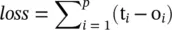

where p is the number of supervised nodes. The learning algorithm is based on a gradient‐descent strategy and is composed of the following steps:

1 The states are iteratively updated by Eq. (5.1)until a time T.They approach the fixed‐point solution of Eq. (5.2)H(T)≈ H.

2 The gradient of weights W is computed from the loss.

3 The weights W are updated according to the gradient computed in the last step.

Directed graphs : Directed edges can yield more information than undirected edges. For example, in a knowledge graph where the edge starts from the head entity and ends at the tail entity, the head entity is the parent class of the tail entity, which suggests we should treat the information propagation process from parent classes and child classes differently. Here, we use two kinds of weight matrix, W pand W c, to incorporate more precise structural information. The propagation rule is [3]