Savo G. Glisic - Artificial Intelligence and Quantum Computing for Advanced Wireless Networks

1 The regularization parameter C can be given by following prescription according to the range of output values of the training data [103] : , where and σy are the mean and the standard deviation of the training data y, and n is the number of training data.

2 v ‐SVR is employed instead of ε ‐SVR, since it is easy to determine of the number of support vectors by the adjustment of v. The adjustment of parameter v can be determined by an asymptotically optimal procedure, and the theoretically optimal value for Gaussian noise is 0.54 [104]. For the kernel parameter Θ′, the k ‐fold cross‐validation method is utilized [104].

Reduced‐set vectors: In order to share the experience, we are interested in constructing Eq. (4.63)such that the original Eq. (4.62)is approximated. In the following, k (x, x i) is written as k ′(x, x i), considering its kernel parameters Θ ′ in Eq. (4.62). Similarly, in Eq. (4.63), ( x j, z ij, Θ j) is replaced by k (x, z i) according to the kernels constructed in the previous paragraph. Then, let G(x) . With this we have

(4.64)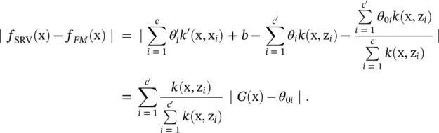

If we let the consequent parameter θ 0ibe G (x 0i), we have

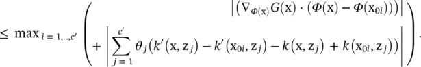
For a smaller upper bound, we assume that Θ ′ = Θ . Then, according to the Cauchy–Schwartz inequality, the right side of the above inequality is simplified to

where , giving

If we use the notation ‖·‖ ∞as 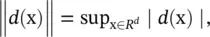we can write

(4.65)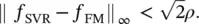

It is expected to obtain a small ρ in order to make a good approximation.

Hybrid learning algorithm : Parameter ρ in Eq. (4.65)is not small enough in many situations. In order to obtain a better approximation, a hybrid learning algorithm including a linear ridge regression algorithm and the gradient descent method can be used to adjust Θ and θ 0iaccording to the experience of Eq. (4.62)[105]. The performance measure is defined as

(4.66)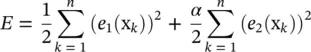

where α is a weighted parameter that defines the relative trade‐off between the squared error loss and the experienced loss, and e 1(x k) = y k− f FM(x k), e 2(x k) = f SVR(x k) − f FM(x k). Thus, the error between the desired output and actual output is characterized by the first term, and the second term measures the difference between the actual output and the experienced output of SVR. Therefore, each epoch of the hybrid learning algorithm is composed of a forward pass and a backward pass which implement the linear ridge regression algorithm and the gradient descent method in E over parameters Θ and θ 0i. Here, θ 0iare identified by the linear ridge regression in the forward pass. In addition, it is assumed that the Gaussian membership function is employed, and thus Θ jis referred as to σ j. Using Eqs. (4.62)and (4.63), and defining

(4.67)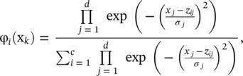

then, at the minimum point of Eq. (4.66)all derivatives with respect to θ 0ishould vanish:

(4.68)

These conditions can be rewritten in the form of normal equations:

(4.69)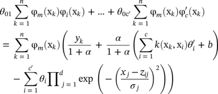

where m = 1, … , c ′. This is a standard problem that forms the grounds for linear regression, and the most well‐known formula for estimating θ = [ θ 01 θ 02⋯ θ 0c′] Tuses the ridge regression algorithm:

(4.70)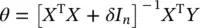

where δ is a positive scalar, and

(4.71)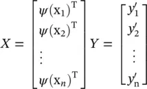

where ,

ψ (x k) = [φ 1(x k), φ 2(x k), ⋯, φ c′(x k)] T, k = 1, … n . In the backward pass, the error rates propagate backward and σ jare updated by the gradient descent method. The derivatives with respect to are calculated from

(4.72)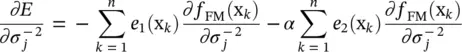

where

(4.73)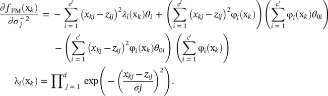

and σ jare updated as

(4.74)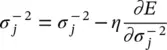

where η is the constant step size.