Savo G. Glisic - Artificial Intelligence and Quantum Computing for Advanced Wireless Networks

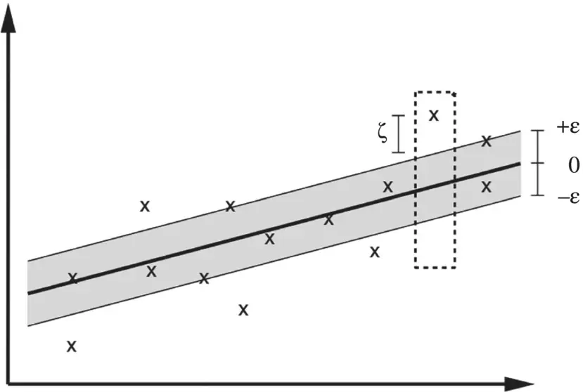
Figure 4.6 Illustration of the soft margin for a linear support vector machine (SVM).

(4.47)

Figure 2.7of Chapter 2is modified to reflect better the definitions introduced in this section and presented as Figure 4.6. Often, the optimization problem, Eq. (4.46), can be solved more easily in its dual formulation. The dual formulation provides also the key for extending SV machine to nonlinear functions.

Lagrange function: The key idea here is to construct a Lagrange function from the objective function ( primal objective function) and the corresponding constraints, by introducing a dual set of variables [95]. It can be shown that this function has a saddle point with respect to the primal and dual variables at the solution. So we have

(4.48)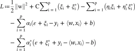

Here, L is the Lagrangian, and η i, α i, are Lagrange multipliers. Hence, the dual variables in Eq. (4.48)have to satisfy positivity constraints, that is, 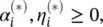where by , we jointly refer to α iand In the saddle point, the partial derivatives of L with respect to the primal variables have to vanish; that is, 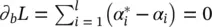, 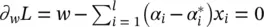and = 0. Substituting these conditions into Eq. (4.48)yields the dual optimization problem:

(4.49)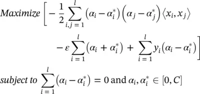

In deriving Eq. (4.49), we already eliminated the dual variables η i, through condition = 0, which can be reformulated as . Equation can be rewritten as , giving

(4.50)

This is the so‐called support vector expansion ; that is, w can be completely described as a linear combination of the training patterns x i. In a sense, the complexity of a function’s representation by SVs is independent of the dimensionality of the input space X , and depends only on the number of SVs. Moreover, note that the complete algorithm can be described in terms of dot products between the data. Even when evaluating f ( x ), we need not compute w explicitly. These observations will come in handy for the formulation of a nonlinear extension.

Computing b : Parameter b can be computed by exploiting the so‐called Karush−Kuhn−Tucker (KKT) conditions stating that at the point of the solution the product between dual variables and constraints has to vanish, giving α i( ε + ξ i− y i+ 〈 w , x i〉 + b ) = 0, , ( C − α i) ξ i= 0 and This allows us to draw several useful conclusions:

1 Only samples (xi, yi) with corresponding lie outside the ε ‐insensitive tube.

2 ; that is, there can never be a set of dual variables αi , that are both simultaneously nonzero. This allows us to conclude that(4.51) (4.52)

In conjunction with an analogous analysis on , we have for b

(4.53)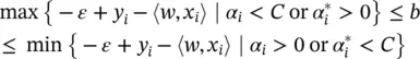

Kernels: We are interested in making the SV algorithm nonlinear. This, for instance, could be achieved by simply preprocessing the training patterns x iby a map Φ : X → F into some feature space F , as already described in Chapter 2, and then applying the standard SV regression algorithm. Let us have a brief look at the example given in Figure 2.8of Chapter 2. We had (quadratic features in ℝ 2) with the map Φ : ℝ 2→ ℝ 3with Φ 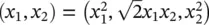. It is understood that the subscripts in this case refer to the components of x ∈ ℝ 2. Training a linear SV machine on the preprocessed features would yield a quadratic function as indicated in Figure 2.8. Although this approach seems reasonable in the particular example above, it can easily become computationally infeasible for both polynomial features of higher order and higher dimensionality.