Savo G. Glisic - Artificial Intelligence and Quantum Computing for Advanced Wireless Networks

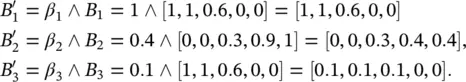
Finally, step 3 gives the overall output fuzzy set:

which is identical to the result from the previous example.

Multivariable systems: So far, the linguistic model was presented in a general manner covering both the single‐input and single‐output (SISO) and multiple‐input and multiple‐output (MIMO) cases. In the MIMO case, all fuzzy sets in the model are defined on vector domains by multivariate membership functions. It is, however, usually more convenient to write the antecedent and consequent propositions as logical combinations of fuzzy propositions with univariate membership functions. Fuzzy logic operators, such as the conjunction, disjunction, and negation (complement), can be used to combine the propositions. Furthermore, a MIMO model can be written as a set of multiple‐input and single‐output (MISO) models, which is also convenient for the ease of notation. Most common is the conjunctive form of the antecedent, which is given by

(4.40)

Note that the above model is a special case of Eq. (4.31), as the fuzzy set A iin Eq. (4.31)is obtained as the Cartesian product of fuzzy sets A ij: A i= A i1× A i2× · · · × A ip. Hence, the degree of fulfillment (step 1 of Algorithm 4.1) is given by

(4.41)

Other conjunction operators, such as the product, can be used. A set of rules in the conjunctive antecedent form divides the input domain into a lattice of fuzzy hyper‐boxes, parallel with the axes. Each of the hyper‐boxes is a Cartesian product‐space intersection of the corresponding univariate fuzzy sets. The number of rules in the conjunctive form needed to cover the entire domain is given by 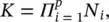where p is the dimension of the input space, and N iis the number of linguistic terms of the i‐ th antecedent variable.

By combining conjunctions, disjunctions‚ and negations, various partitions of the antecedent space can be obtained; the boundaries are, however, restricted to the rectangular grid defined by the fuzzy sets of the individual variables. As an example, consider the rule “If x 1is not A 13and x 2is A 21then …”

The degree of fulfillment of this rule is computed using the complement and intersection operators:

(4.42)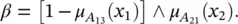

The antecedent form with multivariate membership functions, Eq. (4.31), is the most general one, as there is no restriction on the shape of the fuzzy regions. The boundaries between these regions can be arbitrarily curved and opaque to the axes. Also, the number of fuzzy sets needed to cover the antecedent space may be much smaller than in the previous cases. Hence, for complex multivariable systems, this partition may provide the most effective representation.

Defuzzification: In many applications, a crisp output y is desired. To obtain a crisp value, the output fuzzy set must be defuzzified. With the Mamdani inference scheme, the center of gravity (COG) defuzzification method is used. This method computes the y coordinate of the COG of the area under the fuzzy set B ′:

(4.43)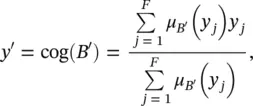

where F is the number of elements y jin Y . The continuous domain Y thus must be discretized to be able to compute the COG.

Consider the output fuzzy set B ′ = [0.2, 0.2, 0.3, 0.9, 1] from the previous example, where the output domain is Y = [0, 25, 50, 75, 100]. The defuzzified output obtained by applying Eq. (4.43)is

The network throughput (in arbitrary units), computed by the fuzzy model, is thus 72.12.

The basic idea: Let {( x 1, y 1), . . . , ( x l, y l)} ⊂ X × ℝ , be a given training data, where X denotes the space of the input patterns (e.g., X = ℝ d). In ε‐SV regression, the objective is to find a function f ( x ) that has at most a deviation of ε from the actually obtained targets y ifor all the training data, and at the same time is as flat as possible. In other words, we do not care about errors as long as they are less than ε, but will not accept any deviation larger than this. We begin by describing the case of linear functions, f , taking the form

(4.44)

where 〈 , 〉 denotes the dot product in X . Flatness in the case of Eq. (4.44)means that one seeks a small w . One way to ensure this is to minimize the norm, that is, ‖ w ‖ 2= 〈 w , w 〉. We can write this problem as a convex optimization problem:

(4.45)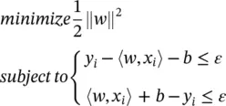

The tacit assumption in Eq. (4.45)was that such a function f actually exists that approximates all pairs ( x i, y i) with ε precision, or in other words, that the convex optimization problem is feasible. Sometimes, the problem might not have a solution for the given ε , or we also may want to allow for some errors. In analogy with the “soft margin” (see Figure 2.7of Chapter 2), one can introduce slack variables ξ i, to cope with possibly infeasible constraints of the optimization problem: Eq. (4.45). So we have

(4.46)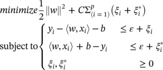

The constant C > 0 determines the trade‐off between the flatness of f and the amount up to which deviations larger than ε are tolerated. This corresponds to dealing with a so‐called ε ‐insensitive loss function | ξ | εdescribed by