Savo G. Glisic - Artificial Intelligence and Quantum Computing for Advanced Wireless Networks

(5.5)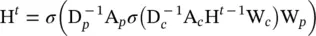

where are the normalized adjacency matrix for parents and children, respectively, and σ denotes a nonlinear activation function.

Heterogeneous graphs : These have several kinds of nodes. The simplest way to process heterogeneous graphs is to convert the type of each node to a one‐hot feature vector that is concatenated with the original feature. GraphInception [4] introduces the concept of metapath into propagation on the heterogeneous graph. With metapath, we can group neighbors according to their node types and distances. For each neighbor group, GraphInception treats it as a subgraph in a homogeneous graph to perform propagation and concatenates the propagation results from different homogeneous graphs to arrive at a collective node representation. In [5], the heterogeneous graph attention network (HAN) was proposed, which utilizes node‐level and semantic‐level attention. The model has the ability to consider node importance and meta‐paths simultaneously.

Graphs with edge information : Here, each edge has additional information like the weight or the type of the edge. There are two ways to handle this kind of graph:

1 We can convert the graph to a bipartite graph where the original edges also become nodes and one original edge is split into two new edges, which means there are two new edges between the edge node and begin/end nodes. The encoder of GS2 (Graph to Sequence) [6] uses the following aggregation function for neighbors:(5.6) where Wr and br are the propagation parameters for different types of edges (relations r), ρ is a nonlinearity, ⊙ stands for the Hadamard product and is the set of neighboring nodes.

2 We can adapt different weight matrices for propagation on different kinds of edges. When the number of relations is very large, r‐GCN (Relational Data with Graph Convolutional Networks) [7] introduces two kinds of regularization to reduce the number of parameters for modeling relations: basis‐ and block‐diagonal‐decomposition. With the basis decomposition, each Wr is defined as follows:(5.7)

Here each W ris a linear combination of basis transformations 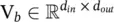with coefficients a rb. In the blockdiagonal decomposition, r‐GCN defines each W rthrough the direct sum over a set of low‐dimensional matrices, which needs more parameters than the first one.

Dynamic graphs : These have a static graph structure and dynamic input signals. To capture both kinds of information, diffusion convolutional recurrent NN (DCRNN) [8] and spatial‐temporal graph convolutional networks (STGCN) [9] first collect spatial information by GNNs, then feed the outputs into a sequence model like sequence‐to‐sequence model or convolutional neural networks (CNNs). On the other hand, structural‐recurrent NN [10] and STGCN [11] collect spatial and temporal messages at the same time. They extend the static graph structure with temporal connections so that they can apply traditional GNNs to the extended graphs.

The propagation step and output step in the model define the hidden states of nodes (or edges). Several major modifications have been made to the propagation step from the original GNN model, whereas in the output step a simple feedforward neural network setting is the most popular. The variants utilize different aggregators to gather information from each node’s neighbors and specific updaters to update nodes’ hidden states.

Convolution has been generalized to the graph domain as well. Advances in this direction are often categorized as spectral approaches and non‐spectral (spatial) approaches. Spectral approaches work with a spectral representation of the graphs.

Spectral network : The spectral network was proposed in Bruna et al. [12]. The convolution operation is defined in the Fourier domain by computing the eigen decomposition of the graph Laplacian. For the basics of these techniques, see Appendix 5.A. The operation can be defined as the multiplication of a signal x ∈ ℝ N(a scalar for each node) with a filter g θ= diag( θ ) parameterized by θ ∈ ℝ N:

(5.8)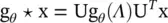

where U is the matrix of the eigenvectors of the normalized graph Laplacian (D is the degree matrix, and A is the adjacency matrix of the graph), with a diagonal matrix of its eigenvalues Λ .

ChebyshevNet [13] truncates g θ( Λ ) in terms of Chebyshev polynomials T k( x ) up to K thorder as

(5.9)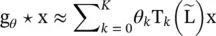

Parameter λ maxdenotes the largest eigenvalue of L. θ ∈ ℝ Kis now a vector of Chebyshev coefficients. The Chebyshev polynomials are defined as T k(x) = 2xT k − 1(x) − T k − 2(x), with T 0(x) = 1 and T 1(x) = x. It can be observed that the operation is K ‐localized since it is a K th‐order polynomial in the Laplacian.

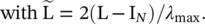
Graph convolutional network (GCN) [14] : This limits the layer‐wise convolution operation to K = 1 to alleviate the problem of overfitting on local neighborhood structures for graphs with very wide node degree distributions. By approximating λ max≈ 2, the equation simplifies to

(5.10)

with two free parameters and . After constraining the number of parameters with , we get